Pandas tutorial (A complete guide with examples and notebook)

Pandas is an open-source Python library that provides a rich collection of data analysis tools for working with datasets. It borrows most of its functionality from the NumPy library. Therefore, we advise that you go through our NumPy tutorial first.

As we dive into familiarizing ourselves with Pandas, it is good first to know why Pandas is helpful in data science and machine learning:

• Pandas provides an efficient way to explore data.
• Has features that help in handling missing data.
• Supports multiple file formats like CSV, JSON, Excel, etc.
• It can efficiently merge a variety of datasets for smooth data analysis.
• Provides tools to read and write data while analyzing.

Setting up Pandas

The quickest way to use Pandas is to download and install the Anaconda Distribution. The Anaconda distribution of Python ships with Pandas and various data science packages.

If you have Python and pip installed, run pip install pandasfrom your terminal or cmd.

pip install pandas

To start using Pandas, you need to import it:

import pandas as pd

Now let's explore some data.

Pandas data structures

Pandas has two prime data structures, Series and DataFrame. These two data structures are built on NumPy arrays, making them fast for data analysis.

A Series is a one-dimensional labeled array structure that we can view as a column in an excel sheet in most cases.

A DataFrame is a two-dimensional array structure and is mostly represented as a table.

Creating and retrieving data from a Pandas Series

We can convert basic Python data structures like lists, tuples, dictionaries, and a NumPy arrays into a Pandas series. The series has row labels which are the index.

We construct a Pandas Series using pandas.Series( data, index, dtype, copy) constructor where:

• data is either a list, ndarray, tuple, etc.
• index is a unique and hashable value.
• dtype is the data type.
• copy copies data.

import numpy as np
import pandas as pd

sample_list_to_series = pd.Series([300, 240, 160]) # pass in the python list into Series method
print(sample_list_to_series)
'''
0    300
1    240
2    160
dtype: int64
'''
sample_ndarray_to_series = pd.Series(np.array([90, 140, 80])) # pass the numpy array in the Series method
print(sample_ndarray_to_series)
'''
0     90
1    140
2     80
dtype: int64
'''

The values in the series have been labeled with their index numbers, that is, the first value with index 0, the second with index 1, and so on. We can use these index numbers to retrieve a value from the series.

import pandas as pd
...
print(sample_list_to_series[1])
# 240
print(sample_ndarray_to_series[2])
# 80

When working with series data, it is not necessary that we only work with the default index assigned to each value. We can label each of these values as we want by using the index argument.

import numpy as np
import pandas as pd

sample_list_to_series = pd.Series([300, 240, 160], index = ['Ninja_HP', 'BMW_HP', 'Damon_HP'])
print(sample_list_to_series)
'''
Ninja_HP    300
BMW_HP      240
Damon_HP    160
dtype: int64
'''
sample_ndarray_to_series = pd.Series(np.array([90, 140, 80]), index = ['valx', 'valy', 'valz'])
print(sample_ndarray_to_series)
'''
valx     90
valy    140
valz     80
dtype: int64
'''

Then we can retrieve the data with the index label values like this:

print(sample_list_to_series['BMW_HP])
# 240
print(sample_ndarray_to_series['valy'])
# 140

Note that with dictionaries, we don't need to specify the index. Since a Python dictionary is composed of key-value pairs, the keys will be used to create the index for the values.

import pandas as pd

sample_dict = {'Ninja_HP': 300, 'BMW_HP': 240, 'Damon_HP': 160}
print(pd.Series(sample_dict))
'''
Ninja_HP    300
BMW_HP      240
Damon_HP    160
dtype: int64
'''

To retrieve multiple data, we use a list of index label values like this:

print(sample_list_to_series[['Ninja_HP', 'Damon_HP']])

'''
Ninja_HP    300
Damon_HP    160
dtype: int64
'''

Indexing

Creating and retrieving data from a Pandas DataFrame

Data in a DataFrame is organized in the form of rows and columns. We can create a DataFrame from lists, tuples, NumPy arrays, or from a series. However, in most cases, we create it from dictionaries using pandas.DataFrame( data, index, columns, dtype, copy) constructor, where columns are for column labels.

Creating a DataFrame from a dictionary of lists

Note that the lists used should be the same length; otherwise, an error will be thrown.

import pandas as pd

dict_of_lists = {'model' : ['Bentley', 'Toyota', 'Audi', 'Ford'], 'weight' : [1400.8, 2500, 1600, 1700]}
data_frame = pd.DataFrame(dict_of_lists)
print(data_frame)
'''
     model  weight
0  Bentley  1400.8
1   Toyota  2500.0
2     Audi  1600.0
3     Ford  1700.0
'''

If we pass no index specifications in the DataFrame method, the default index is passed in range(n), where n is the length of the list. In most cases, this is not what we want, so we will create an indexed DataFrame.

import pandas as pd

dict_of_lists = {'Model' : ['Bentley', 'Toyota', 'Audi', 'Ford'], 'Weight' : [1400.8, 2500, 1600, 1700]}
indexed_data_frame = pd.DataFrame(dict_of_lists, index = ['model_1', 'model_2', 'model_3', 'model_4'])
print(indexed_data_frame)
'''
           Model  Weight
model_1  Bentley  1400.8
model_2   Toyota  2500.0
model_3     Audi  1600.0
model_4     Ford  1700.0
'''

Creating a DataFrame from a dictionary of Series

import pandas as pd

dict_of_series = {'HP': pd.Series([300, 240, 160], index = ['Ninja', 'BMW', 'Damon']), 'speed' : pd.Series(np.array([280, 300, 260, 200]), index = ['Ninja', 'BMW', 'Damon', 'Suzuki'])}
print(pd.DataFrame(dict_of_series))
'''
           HP  speed
BMW     240.0    300
Damon   160.0    260
Ninja   300.0    280
Suzuki    NaN    200
'''

In the HP series, there is no label for Suzuki passed; hence, we get NaN appended in the results.

Selecting, adding, and deleting columns

Accessing a column is as simple as accessing a value from a Python dictionary. We pass in its name to the DataFrame, which returns the results in the form of a pandas.Series.

import pandas as pd

dict_of_lists = {'Model' : ['Bentley', 'Toyota', 'Audi', 'Ford'], 'Weight' : [1400.8, 2500, 1600, 1700]}
indexed_data_frame = pd.DataFrame(dict_of_lists, index = ['model_1', 'model_2', 'model_3', 'model_4'])
print(indexed_data_frame['Weight']) # get the weights column
'''
model_1    1400.8
model_2    2500.0
model_3    1600.0
model_4    1700.0
Name: Weight, dtype: float64
'''

We can add a column to an existing DataFrame using a new Pandas Series. In the example below, we are adding the fuel consumption for each bike in the DataFrame.

import pandas as np

dict_of_series = {'HP': pd.Series([300, 240, 160], index = ['Ninja', 'BMW', 'Damon']), 'speed' : pd.Series(np.array([280, 300, 260, 200]), index = ['Ninja', 'BMW', 'Damon', 'Suzuki'])}
bikes_data_df= pd.DataFrame(dict_of_series)
#add column of fuel consumption
bikes_data_df['Fuel Consumption'] = pd.Series(np.array(['27Km/L', '24Km/L', '30Km/L', '22Km/L']), index = ['Ninja', 'BMW', 'Damon', 'Suzuki']) #add column of fuel consumption
print(bikes_data_df)
'''
           HP  speed Fuel Consumption
BMW     240.0    300           24Km/L
Damon   160.0    260           30Km/L
Ninja   300.0    280           27Km/L
Suzuki    NaN    200           22Km/L
'''

Columns can also be deleted from the DataFrame. To do this, we can either use the pop or delete functions. Let's remove the speed and Fuel Consumption columns from the bike DataFrame.

import numpy as np
...
# using pop function
bikes_data_df.pop('speed')
print(bikes_data_df)
'''
           HP Fuel Consumption
BMW     240.0           24Km/L
Damon   160.0           30Km/L
Ninja   300.0           27Km/L
Suzuki    NaN           22Km/L
'''
#using delete function
del bikes_data_df['Fuel Consumption']
print(bikes_data_df)
'''
           HP
BMW     240.0
Damon   160.0
Ninja   300.0
Suzuki    NaN
'''

Selecting, adding, and deleting rows

Pandas has accessor operators loc and iloc which we can use to access rows in a DataFrame.

iloc does index-based selection. It selects a row based on its integer position in the DataFrame. In the following code, we select data on the second row in the DataFrame.

import pandas as np

dict_of_series = {'HP': pd.Series([300, 240, 160], index = ['Ninja', 'BMW', 'Damon']), 'speed' : pd.Series(np.array([280, 300, 260, 200]), index = ['Ninja', 'BMW', 'Damon', 'Suzuki'])}
bikes_data_df= pd.DataFrame(dict_of_series)
bikes_data_df.iloc[1]
'''
HP       160.0
speed    260.0
Name: Damon, dtype: float64
'''

loc does label-based selection. It selects a row based on the data index value rather than the position. Let's choose data from the row with the label 'BMW'.

import pandas as pd

dict_of_series = {'HP': pd.Series([300, 240, 160], index = ['Ninja', 'BMW', 'Damon']), 'speed' : pd.Series(np.array([280, 300, 260, 200]), index = ['Ninja', 'BMW', 'Damon', 'Suzuki'])}
bikes_data_df= pd.DataFrame(dict_of_series)
bikes_data_df.loc['BMW']
'''
HP       240.0
speed    300.0
Name: BMW, dtype: float64
'''

We can add a new row using the append function to the DataFrame. Observe that the new rows will be added to the end of the original DataFrame.

import pandas as pd

sample_dataframe1 = pd.DataFrame([['Ninja',280],['BMW',300],['Damon',200]], columns = ['Model','Speed'])
sample_dataframe2 = pd.DataFrame([['Suzuki', 260], ['Yamaha', 180]], columns = ['Model','Speed'])
sample_dataframe1 = sample_dataframe1.append(sample_dataframe2)
print(sample_dataframe1)
'''
    Model  Speed
0   Ninja    280
1     BMW    300
2   Damon    200
0  Suzuki    260
1  Yamaha    180
'''

Reading and analyzing data with Pandas

We've looked at two major Pandas data structures which are the Series and DataFrame. You've also learned how to create them by hand. However, nearly every time we will not need to create this data by ourselves rather, we will be carrying out data analysis from already existing data.

There are numerous formats in which data can be stored, but in this article, we shall look at the following kinds of data formats:

• Comma Separated Values(CSV) file.
• JSON file.
• SQL database file.
• Excel file.

Reading and analyzing data from a CSV file

Let's use the Melbourne housing market dataset from Kaggle. We will download the data into our Jupyter notebook using the API provided by Kaggle. The dataset is a zip file, so we need to unzip it.

We have used the Linux and installation commands starting with “!” as shown in the image below.

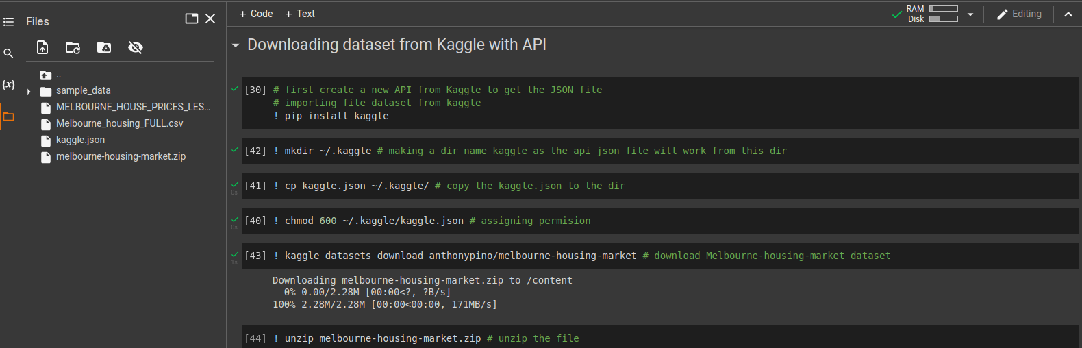
To load the data from the CSV file, we use pd.read_csv().

import pandas as pd

melbourne_data = pd.read_csv('/content/Melbourne_housing_FULL.csv')
melbourne_data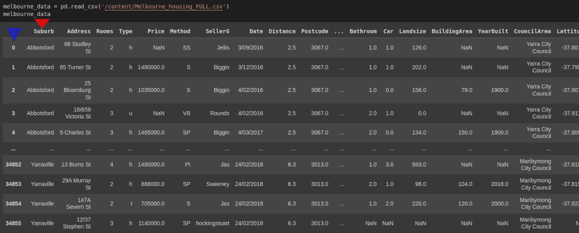

The results show that Pandas created its own column of indexes(blue triangle) despite the CSV file having its own column of indexes(red triangle). To make Pandas use the CSV's column of indexes, we specify the index_col.

import pandas as pd

melbourne_data = pd.read_csv('/content/Melbourne_housing_FULL.csv', index_col=0)
melbourne_data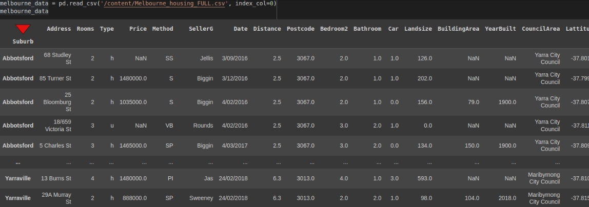

Aside: If you wish to return the index to the normal one(0, 1...etc) you can use the reset_index() method. This method will reset the DataFrame's index and use the default.

melbourne_data.reset_index()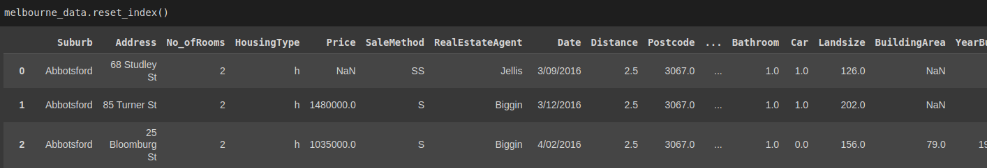

Note that the suburb index we set is returned as a column. However, let's proceed with an indexed DataFrame.

Since the data is huge and represented in a DataFrame, Pandas returns the first five rows and the last five rows. We can check how large this data is using the shape attribute.

import pandas as pd

...
print(melbourne_data.shape)
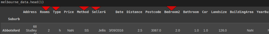
# (34857, 21)

The DataFrame has about 34857 records(rows) and 21 columns. It's possible to examine any number of records we want using the head() method. By default, this method will display the first five records.

import pandas as pd

...
melbourne_data.head()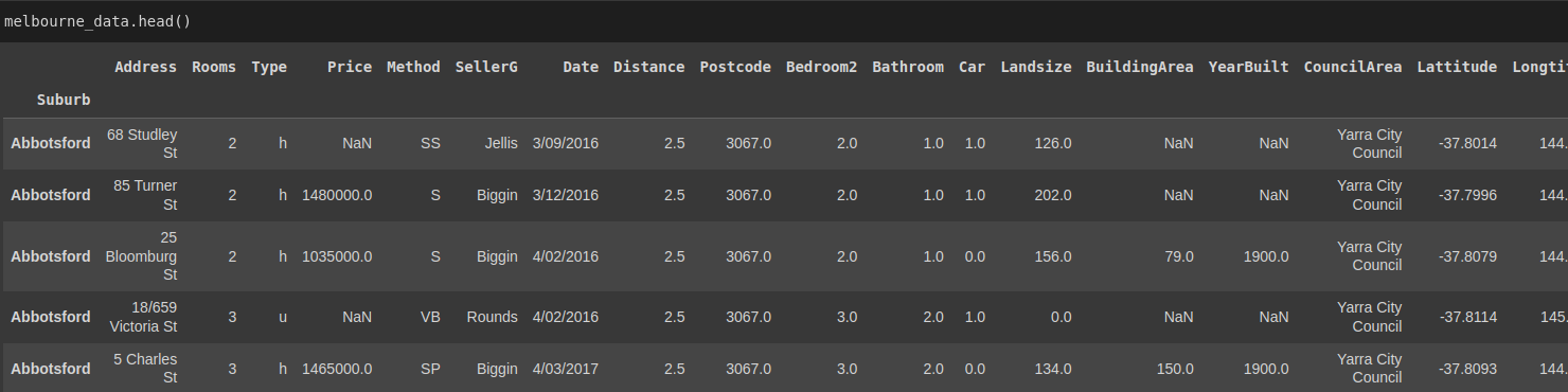

Specifying the number of records we want.

import pandas as pd

...
melbourne_data.head(3) # returns the first three records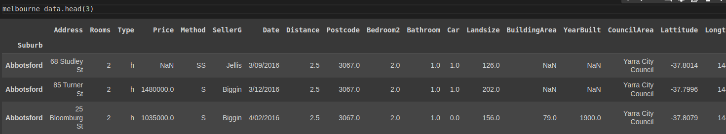

We can also use thetail() method to examine the last n number of rows/records. By default, it returns the last five records.

import pandas as pd

...
melbourne_data.tail(3) # returns the last three records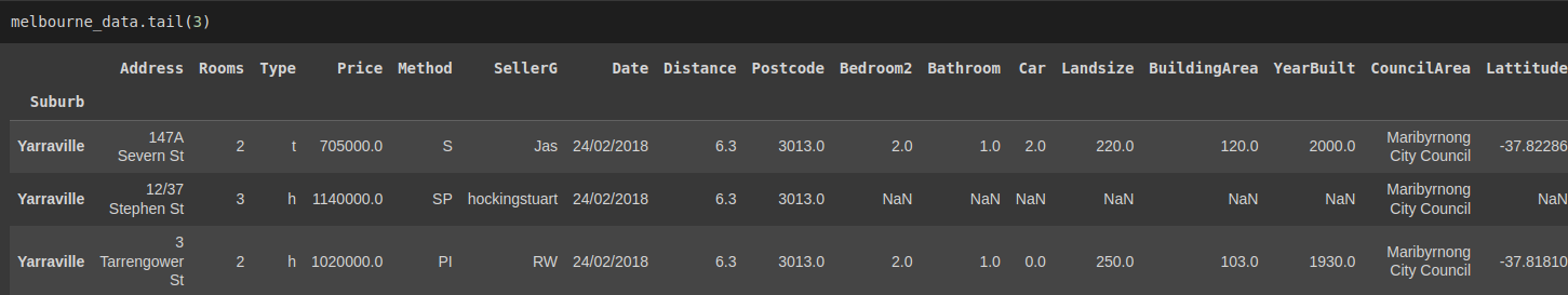

To get more information about the dataset, we can use the info() method. This method prints the number of entries in the dataset and the data type in each column.

import pandas as pd
...
print(melbourne_data.info())
'''
<class "pandas.core.frame.DataFrame">
Index: 34857 entries, Abbotsford to Yarraville
Data columns (total 20 columns):
 #   Column         Non-Null Count  Dtype  
---  ------         --------------  -----  
 0   Address        34857 non-null  object 
 1   Rooms          34857 non-null  int64  
 ...
 18  Regionname     34854 non-null  object 
 19  Propertycount  34854 non-null  float64
dtypes: float64(12), int64(1), object(7)
memory usage: 5.6+ MB
None
'''

Reading data from a JSON file

Let's create a simple JSON file using Python and read it using Pandas.

import json

# creating a simple JSON file
car_data ={
        'Porsche': {
        'model': '911',
        'price': 135000,
        'wiki': 'http://en.wikipedia.org/wiki/Porsche_997',
        'img': '2004_Porsche_911_Carrera_type_997.jpg'
    },'Nissan':{        
        'model': 'GT-R',
        'price': 80000,
        'wiki':'http://en.wikipedia.org/wiki/Nissan_Gt-r',
        'img': '250px-Nissan_GT-R.jpg'
    },'BMW':{
        'model': 'M3',
        'price': 60500,
        'wiki':'http://en.wikipedia.org/wiki/Bmw_m3',
        'img': '250px-BMW_M3_E92.jpg'
    },'Audi':{
        'model': 'S5',
        'price': 53000,
        'wiki':'http://en.wikipedia.org/wiki/Audi_S5',
        'img': '250px-Audi_S5.jpg'
    },'Audi':{
        'model': 'TT',
        'price': 40000,
        'wiki':'http://en.wikipedia.org/wiki/Audi_TT',
        'img': '250px-2007_Audi_TT_Coupe.jpg'
    }
}
jsonString = json.dumps(car_data)
jsonFile = open("cars.json", "w")
jsonFile.write(jsonString)
jsonFile.close()

Now we have a cars.json file.

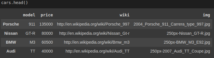
To read data from the JSON file, we use pd.read_json(). Pandas will automatically convert the object of dictionaries into a DataFrame and define the column names separately.

import pandas as pd

pd.read_json('/content/cars.json')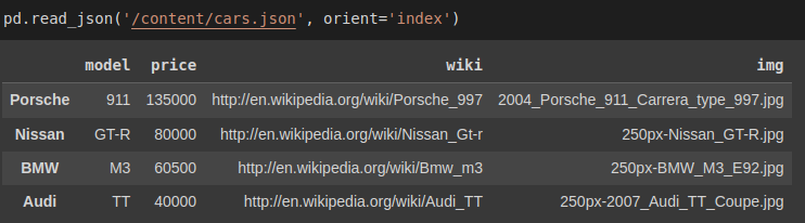

To analyze the data you can apply the info, head(), and tail() methods like we did for CSV files.

Reading data from a SQL database

Let's create a database with python sqlite3 to demonstrate this. Pandas has read_sql_query() method that will convert the data into a DataFrame.

First, we connect to SQLite, create a table, and insert values.

import sqlite3
conn = sqlite3.connect('vehicle_database') 
c = conn.cursor()
# let's create a table and insert values with sqlite3
c.execute('''
          CREATE TABLE IF NOT EXISTS vehicle_data
          ([vehicle_id] INTEGER PRIMARY KEY, [vehicle_model] TEXT, [weight] INTEGER, [color] TEXT)
          ''')                     
conn.commit()
# insert values into tables
c.execute('''
          INSERT INTO vehicle_data (vehicle_id, vehicle_model, weight, color)
                VALUES
                (1,'Bentley',1400,'Blue'),
                (2,'Toyota',2500,'Green'),
                (3,'Audi',1600,'Black'),
                (4,'Ford',1700,'White')
          ''')
conn.commit()

In the vehicle database, we have a table called vehicle_data. We will pass the SELECT statement and the conn variable to read from that table.

cars_df = pd.read_sql_query("SELECT * FROM vehicles", conn)
cars_df.set_index('vehicle_id') # set index to vehicle_id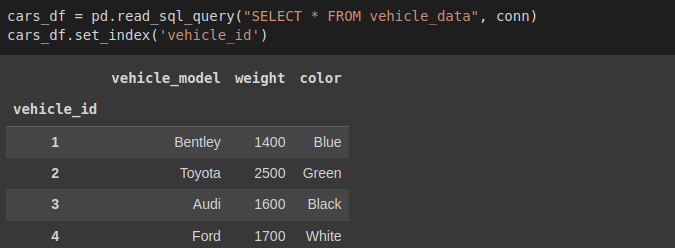

Reading data from an Excel file

We can create a sample excel file to demonstrate how to read data from Excel files. Make sure to install the XlsxWriter module.

pip install xlsxwriter

import xlsxwriter
workbook = pd.ExcelWriter('students.xlsx', engine='xlsxwriter')
workbook.save()

try:
  df = pd.DataFrame({'stud_id': [1004, 1007, 1008, 1100],
      'Name': ['Brian', 'Derrick', 'Ann', 'Doe'],
      'Age': [24, 26, 22, 25]})
  workbook = pd.ExcelWriter('students.xlsx', engine='xlsxwriter')
  df.to_excel(workbook, sheet_name='Sheet1', index=False)
  workbook.save()
except:
  print('Excel sheet exists!')

We have created an Excel file called students.xlsx. To read data from an Excel file we use read_excel() method.

stud_data = pd.read_excel('/content/students.xlsx')
stud_data.set_index('stud_id')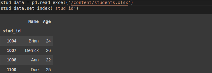

Cleaning data

In data science, we extract insights from huge volumes of raw data. This raw data may contain irregular and inconsistent values, leading to garbage analysis and less useful insights. In most cases, the initial steps of obtaining and cleaning data may constitute 80% of the job; thus, if you plan to step into this field, you must learn how to deal with messy data.

Data cleaning removes wrong, corrupted, incorrectly formatted, duplicate, or incomplete data within a dataset.

In this section, we will cover the following:

• Dropping unnecessary columns in the dataset.
• Removing duplicates.
• Finding and filling missing values in the DataFrame.
• Changing the index of the DataFrame.
• Renaming columns of a DataFrame.

Let's use the Melbourne housing market dataset we imported from Kaggle. First, shuffle the DataFrame to get rows with different indexes. To reproduce the same shuffled data each time, we are using a random_state.

import pandas as pd

...
shuffled_melbourne_data = melbourne_data.sample(frac=1, random_state=1) # produce the same shuffled data each time
shuffled_melbourne_data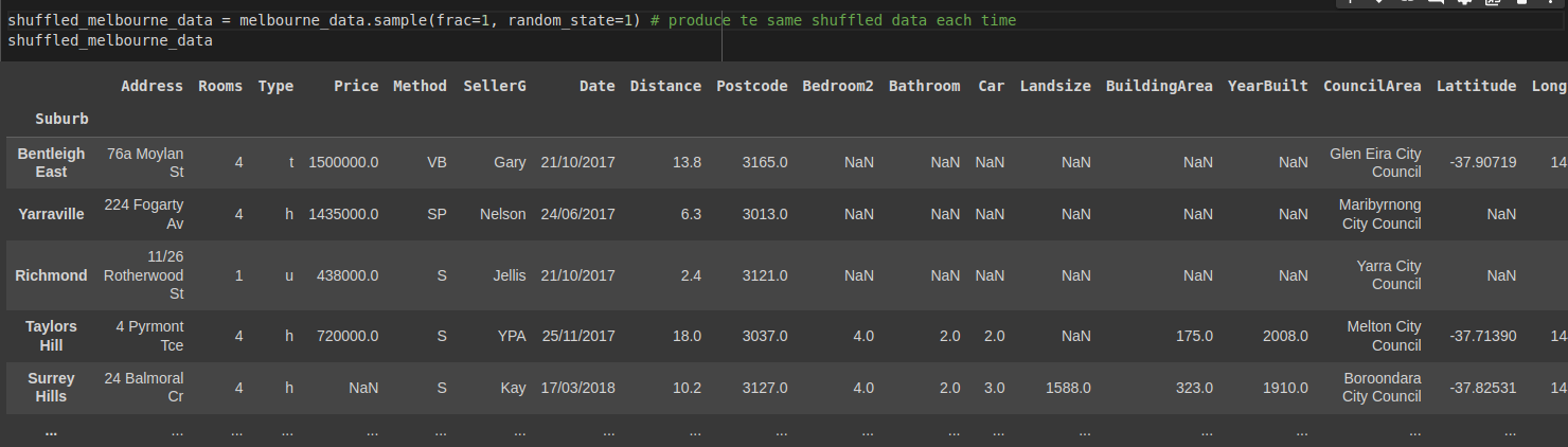

Dropping unnecessary columns in the dataset

Suppose that in the DataFrame we want to get insights about:

• Which suburbs are the best to buy in?
• Suburbs that are value for money?
• Where's the expensive side of town?
• Where to buy a two bedroom unit?

We might need all other columns except:

• Method
• SellerG
• Date
• Bathroom
• Car
• Landsize
• BuildingArea
• YearBuilt

Pandas has a drop() method to remove these columns.

import pandas as pd
...
# Define a list names of all the columns we want to drop
columns_to_drop = ['Method',
                   'SellerG',
                   'Date',
                   'Bathroom',
                   'Car',
                   'Landsize',
                   'BuildingArea',
                   'YearBuilt']
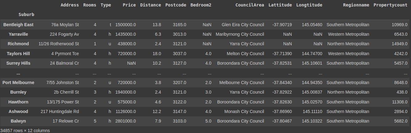
shuffled_melbourne_data.drop(columns = columns_to_drop, inplace=True, axis=1)
shuffled_melbourne_data

Columns dropped!

Finding and removing duplicates

The duplicated() method returns boolean values in a column format. False values mean that no data has been duplicated.

import pandas as pd
...
print(shuffle_melbourne_data.duplicated)
'''
Suburb
Bentleigh East    False
                  ...  
Balwyn            False
Length: 34857, dtype: bool
'''

Checking for duplicates this way can be done for small DataFrames. For huge DataFrames, as we have, it is impossible to check against each value individually. So we will chain the any() method to duplicated().

import pandas as pd
...
print(shuffle_melbourne_data.duplicated.any())
# True

The any() method returns True, which means we have some duplicates in our DataFrame. To remove them, we will use the drop_duplicates() method.

shuffled_melbourne_data.drop_duplicates(inplace=True) # remove dupicates
shuffled_melbourne_data.duplicated().any() # Checking returns False
# False

Finding and filling missing values in the DataFrame.

We have four methods we can use to check for missing/null values. They are:

• isnull() – returns a dataset with boolean values.

shuffled_melbourne_data.isna()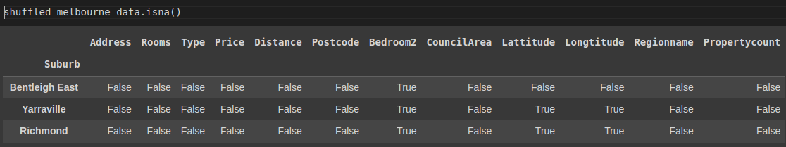

• isna() – similar to isnull().
• isna().any() – returns a column format of boolean values.

shuffled_melbourne_data.isna().any()

'''
Address          False
Rooms            False
				 ...
Propertycount     True
dtype: bool
'''

• isna().sum() – returns a column-wise total of all nulls available.

shuffled_melbourne_data.isna().sum()

'''
Address             0
				...
Price            7580
Distance            1
				...
Propertycount       3
dtype: int64
'''

There are two ways we can deal with missing values:

1. By removing the rows that contain the missing values.

We use the dropna() method to drop the rows. But we will not drop the rows in our dataset yet.

shuffled_melbourne_data.dropna(inplace=True) # removes all rows with null values

2. By replacing the empty cells with new values.

We can decide to replace all the null values with a value using the fillna() method. It has the syntax DataFrame.fillna(value, method, axis, inplace, limit, downcast) where the value can be a dictionary that takes the column names as key.

import pandas as pd

...
shuffled_melbourne_data.fillna({'Price':1435000, 'Distance':13, 'Postcode':3067, 'Bedroom2': 2, 'CouncilArea': 'Yarra City Council'}, inplace=True)
print(shuffled_melbourne_data.isna().sum())
'''
Address             0
Rooms               0
Type                0
Price               0
Distance            0
Postcode            0
Bedroom2            0
CouncilArea         0
Lattitude        7961
Longtitude       7961
Regionname          3
Propertycount       3
dtype: int64
'''

We have successfully replaced empty values specified columns in the dictionary inside the fillna() method.

Changing the index of the DataFrame

While working with data, a uniquely valued field as the data's index is usually desired. For instance, in our cars.json dataset, it can be assumed that when a person searches for a car record, they will probably search it via its Model(Values in the Model column).

Checking if the model column has unique values returns True thus, we will replace the existing index with this column using set_index:

print(cars['model'].is_unique)
# True

cars.set_index('model', inplace=True)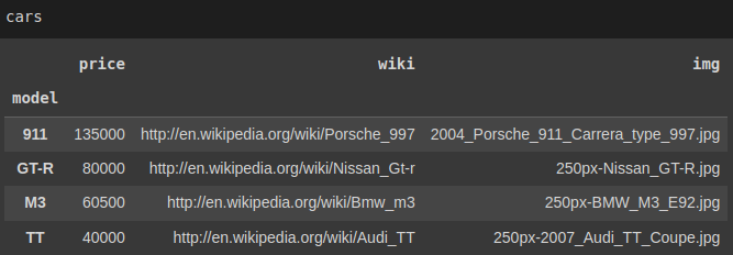

Now it is possible to access each record directly with loc[]

print(cars['M3']

'''
price                                  60500
wiki     http://en.wikipedia.org/wiki/Bmw_m3
img                     250px-BMW_M3_E92.jpg
Name: M3, dtype: object
'''

Renaming columns of a DataFrame

Sometimes you may want to rename columns in your data for better interpretation, maybe because some names are not easy to understand. To do this, you can use the DataFrame's rename() method and pass in a dictionary where the key is the current column name and the value is the new name.

Let's use the original Melbourne DataFrame, where no column has been removed. We may want to rename:

• Room to No_ofRooms.
• Type to HousingType.
• Method to SaleMethod
• SellerG to RealEstateAgent.
• Bedroom2 to No_ofBedrooms.

# Use initial Melbourne DataFrame
#Create a dictionary of columns to rename. Value is the new name
columns_to_rname = {
    'Rooms': 'No_ofRooms',
    'Type': 'HousingType',
    'Method': 'SaleMethod',
    'SellerG': 'RealEstateAgent',
    'Bedroom2': 'No_ofBedrooms'
}
melbourne_data.rename(columns=columns_to_rename, inplace=True)
melbourne_data.head()

Pandas finding relationships(correlations)

Pandas has a method corr() that enables us to find the relationship between each column in our data set.

The method returns a table representing the relationship between two columns. The values vary from -1 to 1, where -1 is a negative correlation and 1 is a perfect one. It will automatically ignore any null values and non-numeric values in the dataset.

shuffled_melbourne_data.corr()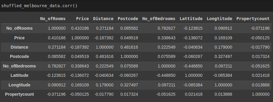

Descriptive statistics

There exist methods in Pandas DataFrames and Series to carry out summary statistics. These methods include: mean, median, max, std, sum() and min.

For instance, we could find the mean for Price in our DataFrame.

shuffled_melbourne_data['Price'].mean()
# 1134144.8576355954
# Or for all columns
No_ofRooms       3.031071e+00
Price            1.134145e+06
				 ...
Propertycount    7.570273e+03
dtype: float64

The describe() method gives an overview of the basic statistics for all the attributes in our data.

shuffled_melbourne_data.describe()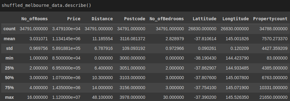

Pandas groupby operation to split, aggregate, and transform data

The Pandas groupby() function enables us to reorganize data. It simply splits data into groups categorized using some criteria and returns a dict of DataFrame objects.

Split data into groups

Let's split our shuffled Melbourne data into groups according to the number of bedrooms. To view the groups, we use thegroups attribute.

grouped_melb_data = shuffled_melbourne_data.groupby('No_ofBedrooms')
grouped_melb_data.groups
'''
{1.0: ['Hawthorn', 'St Kilda'], 2.0: ['Bentleigh East', 'Yarraville', 'Richmond', 'Mill Park', 'Southbank', 'Surrey Hills', 'Caulfield North', 'Reservoir', 'Mulgrave', 'Altona', 'Ormond', 'Bonbeach', 'St Kilda', 'South Yarra', 'Malvern', 'Essendon'], 
... 
30.0: ['Burwood']}}
'''

Since the result is a dict and the data is huge; we can use the keys() method to get the keys.

grouped_melb_data.groups.keys()
# dict_keys([0.0, 1.0, 2.0, 3.0, 4.0, 5.0, 6.0, 7.0, 8.0, 9.0, 10.0, 12.0, 16.0, 20.0, 30.0])

We can group multiple columns like:

grouped_melb_data = shuffled_melbourne_data.head(20).groupby(['No_ofBedrooms', 'Price'])
grouped_melb_data.groups.keys()
'''
dict_keys([(1.0, 365000.0), (1.0, 385000.0), (2.0, 380000.0), (2.0, 438000.0), ... (4.0, 1435000.0)])

Use the get_group() method selects a single group.

grouped_melb_data.get_group(2) # select 2 bedrooms group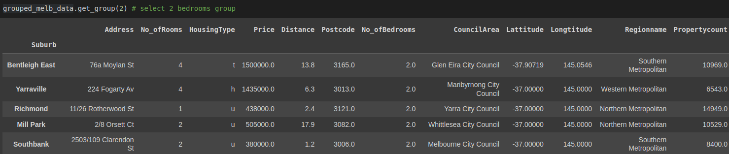

Aggregate data

The aggregate function returns a single collective value for each group. For instance, we want the mean for price in each group. We'll use the aggregate(agg) function.

print(grouped_melb_data['Price'].agg([np.mean]))
'''
                       mean
No_ofBedrooms              
0.0            1.054029e+06
1.0            6.367457e+05
			   ...
30.0           1.435000e+06
'''

Transformation

Pandas has a transform operation that we use with groupby() function. It enables us to summarize data effectively. When we transform a group, we get an indexed object the same size as that being grouped.

For instance, in our dataset, we can get the average prices for each No_ofBedrooms group and combine the results into our dataset for other computations.

Our first approach would be to try to group the data into a new DataFrame and combine it in a multi-step process, then merge the results into the original DataFrame. We would create a new DataFrame with the totals by order and merge it back with the original.

price_means = shuffled_melbourne_data.groupby('No_ofBedrooms')['Price'].mean().rename('MeanPrice').reset_index()
df_1 = shuffled_melbourne_data.merge(price_means)
df_1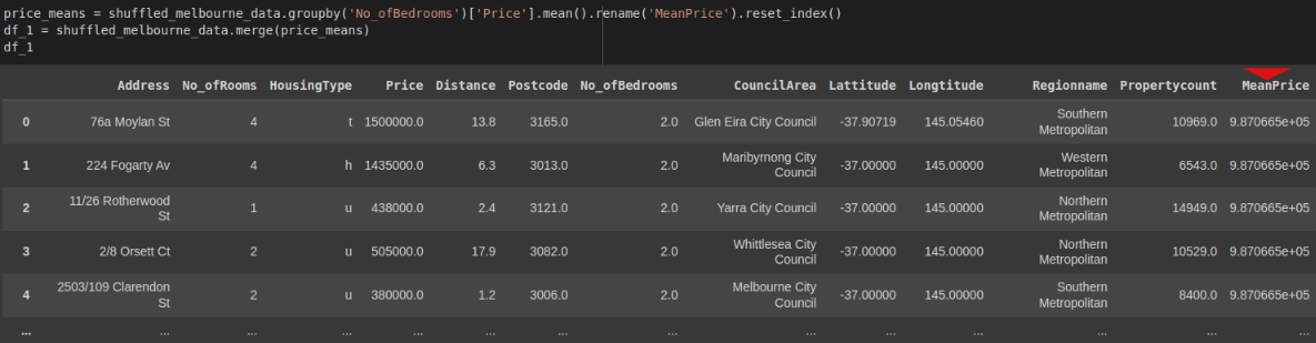

That is quite a hustle, right?

Now let's apply the transform operation to do the same.

shuffled_melbourne_data['MeanPrice'] = shuffled_melbourne_data.groupby('No_ofBedrooms')['Price'].transform('mean')
shuffled_melbourne_data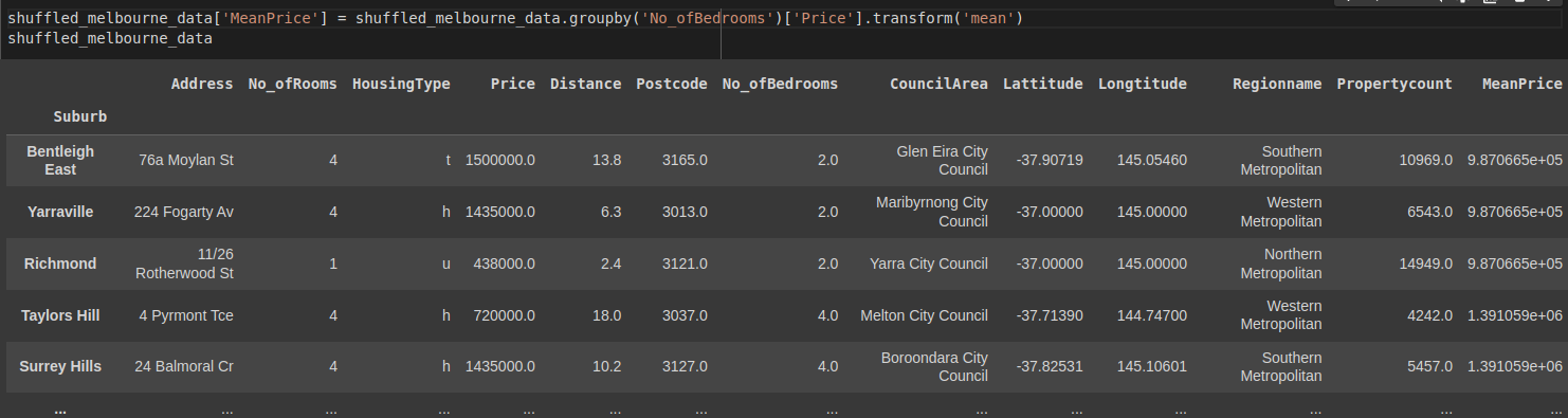

Pandas pivot table

A Pandas pivot table is similar to the groupby operation. It is a common operation for programs that use tabular data like spreadsheets. The difference between the groupby operation and pivot table is that a pivot table takes simple column-wise data as input and groups the entries into a two-dimensional table which gives a multidimensional summarization of the data.

Its syntax is:

pandas.pivot_table(data, values=None, index=None, columns=None, aggfunc=’mean’, fill_value=None, margins=False, dropna=True, margins_name=’All’, observed=False)

Let's create a pivot table:

pivot_tbl = shuffled_melbourne_data.pivot_table(index='HousingType')
pivot_tbl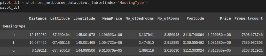

Let's explain the results:

We created a new DataFrame called pivot_tbl from our data with the pivot_table() function. The result is grouped by HousingType as the index. Since no other parameters were specified in the function, the data was aggregated by the mean for each column with numeric data since, by default the aggfunc= parameter returns the mean.

Aggregating the data by specific columns

You can also aggregate data by specific columns. In the example below, we aggregate by the price and room columns.

pivot_tbl = shuffled_melbourne_data.pivot_table(index='HousingType', values=['Price', 'No_ofRooms'])
pivot_tbl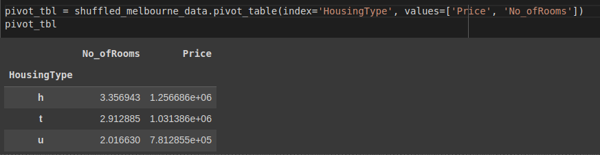

Using aggregation methods in the pivot table

We can change how data is aggregated in the pivot table. We can perform complex analyses with aggregation methods. To use them, we need to use the aggregation function aggfunc.

Let's find the sum of all Propertycount for every region Regionname in our data.

pivot_tbl_sum = shuffled_melbourne_data.pivot_table(index='Regionname', aggfunc='sum', values='Propertycount')
pivot_tbl_sum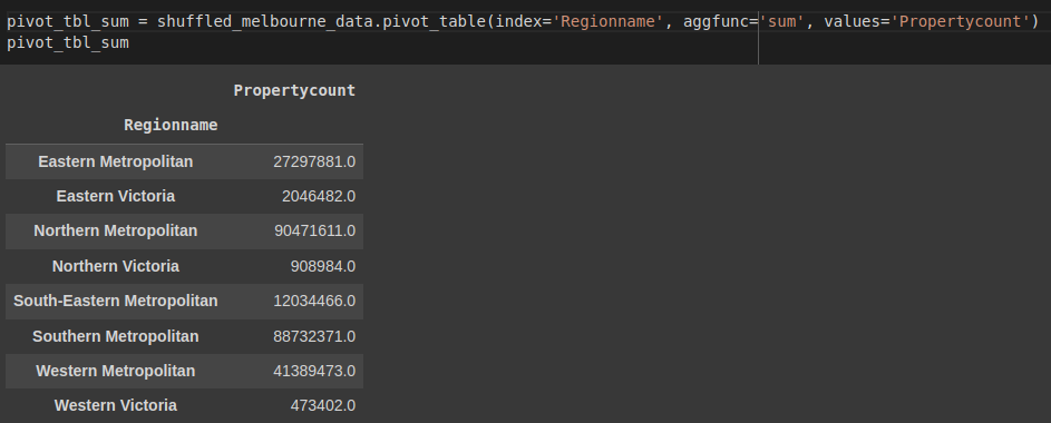

Multiple aggregation methods

To apply multiple aggregation methods, we pass in a list of methods in aggfunc. Let's find the sum and the maximum property count for each region.

pivot_tbl_sum_max = shuffled_melbourne_data.pivot_table(index='Regionname', aggfunc=['sum', 'max'], values='Propertycount')
pivot_tbl_sum_max

Specifying aggregation method for each column

We can pass a dictionary containing the column as the key and the aggregate function as the value.

pivot_tbl = shuffled_melbourne_data.pivot_table(index='Regionname', values=['Price', 'Propertycount'], aggfunc={'Price':'sum', 'Propertycount':'mean'})
pivot_tbl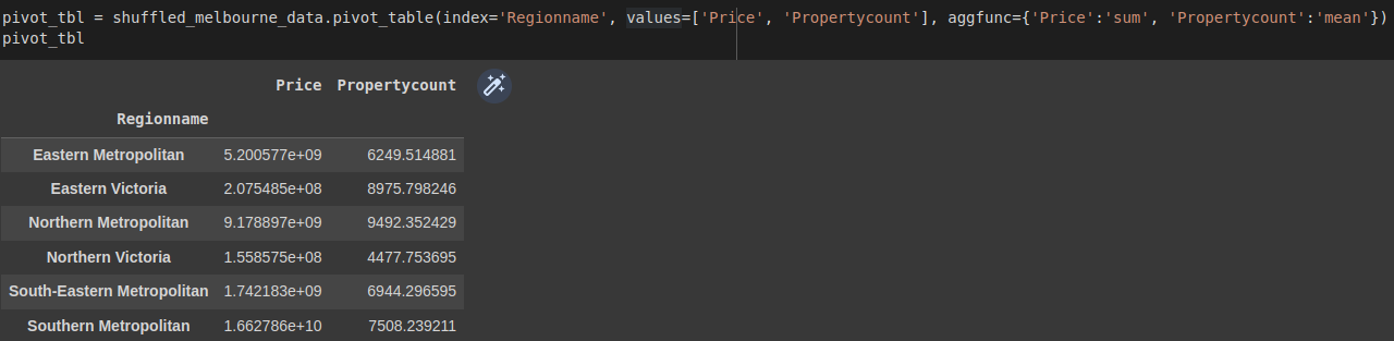

Split data in the pivot table by column with columns

You can add a column to the pivot table with column. This splits the data horizontally while index= splits vertically. In the example below, we split the data by the HousingType.

pivot_tbl = shuffled_melbourne_data.pivot_table(
				index='Regionname',
                values=['Price', 'Propertycount'],
                aggfunc={'Price':'sum', 'Propertycount':'mean'}, 						columns='HousingType'
                )
pivot_tbl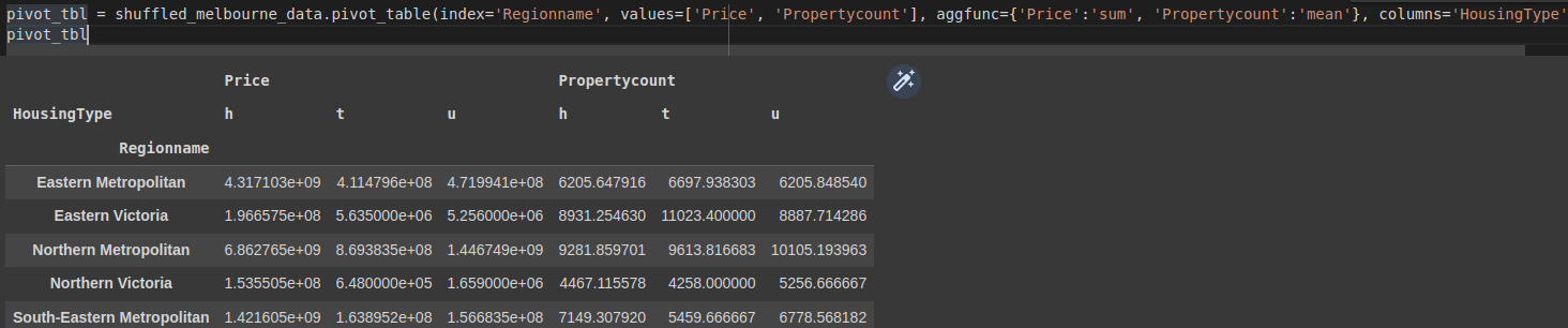

Adding totals to each grouping

Sometimes it's necessary to add totals after aggregating each grouping. We do this using margins=. By default, it is set to False, and its label is set to 'All'. To rename it, we use margin_name=. We can look at the totals of all Propertycount for each region.

pivot_tbl = shuffled_melbourne_data.pivot_table(
					index='Regionname',
                    values='Propertycount',
                    margins=True,
                    margins_name='Totals',
                    aggfunc='sum',
                    columns='HousingType')
pivot_tbl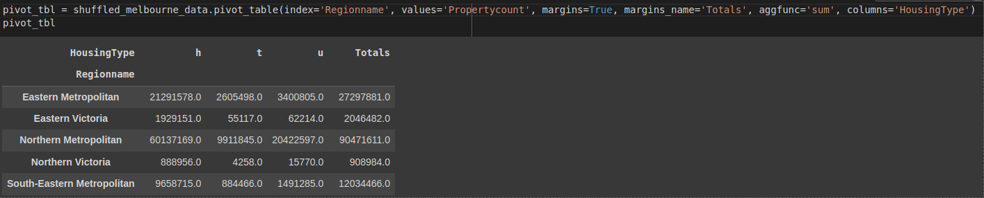

As you might have observed, the pivot table code is easier and more readable as compared to the groupby operation.

Pandas sort DataFrame

Pandas provide a sort_values() method to sort a Pandas DataFrame. The following are types of sorting we can perform:

• Sorting in an ascending order
• Sorting in descending order
• Sorting by multiple columns

Sorting in ascending order

Let's sort the Melbourne data by Price. By default, data is sorted in ascending order.

shuffled_melbourne_data.sort_values(by=['Price'], inplace=True)
shuffled_melbourne_data.head(10)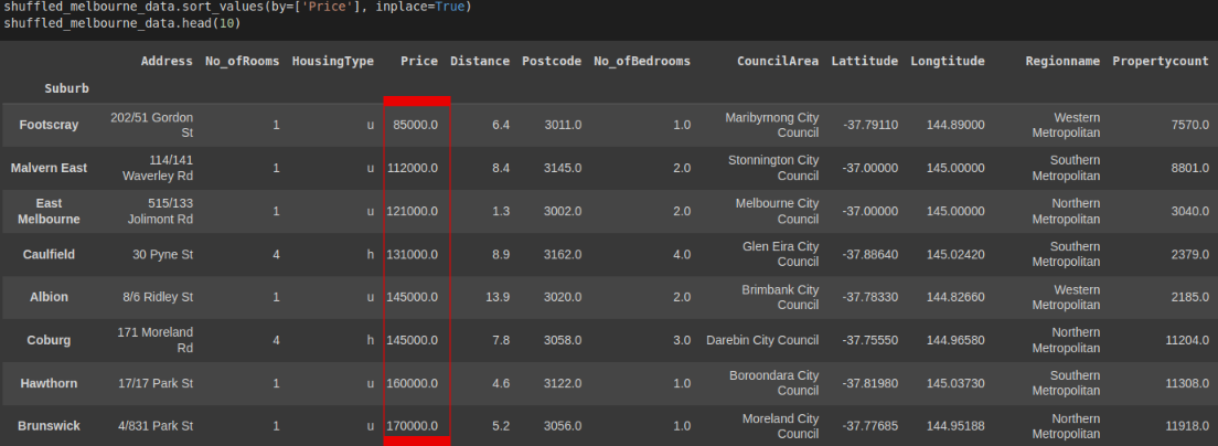

Sorting in descending order

To sort in descending order, we simply need to add the ascending=False condition to the sort_values() method. Let's sort the Melbourne data by Price.

shuffled_melbourne_data.sort_values(by=['Price'], inplace=True, ascending=False)
shuffled_melbourne_data.head(10)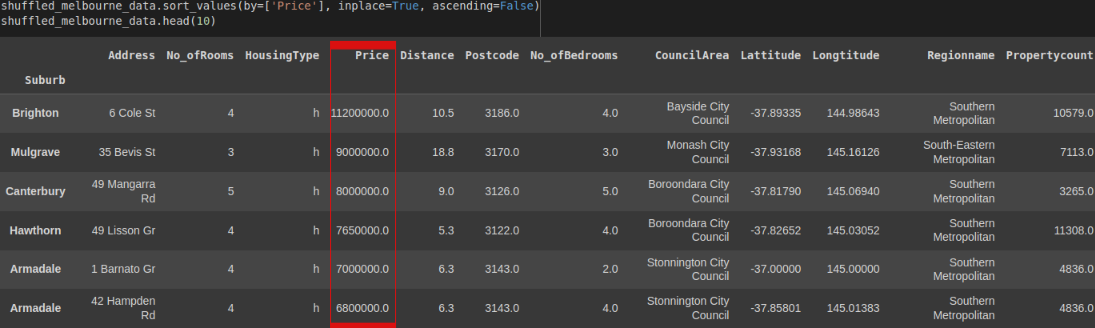

Sorting by multiple columns

We pass a list of columns to the by condition to sort multiple columns. Let's sort the No_ofRooms and price.

shuffled_melbourne_data.sort_values(by=['No_ofRooms','Price'], inplace=True)
shuffled_melbourne_data.head(10)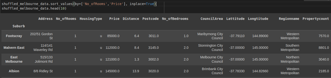

Pandas plotting

Pandas uses the plot() method to create visualizations. Since it integrates with the Matplotlib library, we can use the Pyplot module for these visualizations.

First, let's import matplotlib.pyplot module and give it plt as an alias, then visualize our DataFrame.

import matplotlib.pyplot as plt
plt.rcParams.update({'font.size': 25, 'figure.figsize': (50, 8)}) # set font and plot size to be larger

Scatter Plot

The main purpose of a scatter plot is to check whether two variables are correlated.

shuffled_melbourne_data.plot(kind='scatter', x='No_ofRooms', y='Price', title='Price vs Number of Rooms')
plt.show()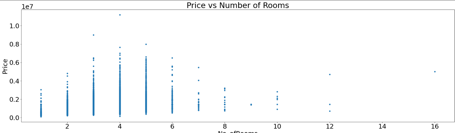

A scatter plot isn’t definitive proof of a connection. For an overview of the correlations between different columns, you can use the corr() method.

Histograms

Histograms help to visualize how values are distributed across a dataset. It gives a visual interpretation of numerical data by showing the number of data points that fall within a specified range of values (called “bins”).

shuffled_melbourne_data['Price'].plot(kind='hist', title='Pricing')
plt.show()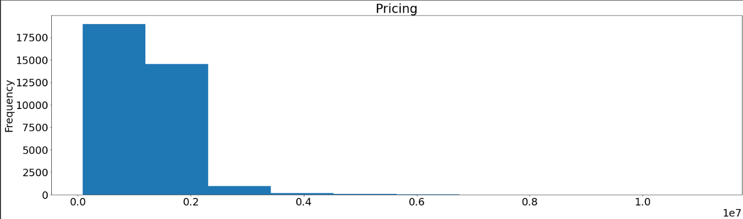

Pie plots

Pie plots show a part-to-whole relationship in your data in ratios.

price_count = shuffled_melbourne_data.groupby('Address')['Price'].sum()
print(price_count) #price totals each group
'''
Address
1 Abercrombie St    1435000.0
1 Aberfeldie Wy      680000.0
                      ...    
9b Stewart St       1160000.0
Name: Price, Length: 34009, dtype: float64
'''
small_groups = price_count[price_count < 1500000]
large_groups = price_count[price_count > 1500000]

small_sums = pd.Series([small_groups.sum()], index=["Other"])
large_groups = large_groups.append(small_sums)

large_groups.iloc[0:10].plot(kind="pie", label="")
plt.show()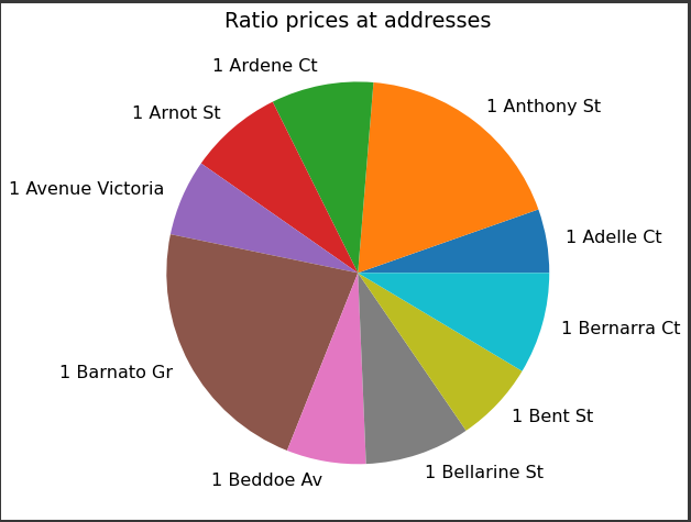

Converting to CSV, JSON, Excel or SQL

After working on your data, you may decide to convert any of the formats to the other. Pandas has methods to do these conversions just as easily as we read the files.

Throughout the entire article, we have used these files:

• Melbourne_housing_FULL.csv file
• cars.json file
• vehicle_database file
• students.xlsx

Convert JSON to CSV

To convert to CSV, we use the df.to_csv() method. So to convert our cars.json file we would do it this way.

cars = pd.read_json('cars.json', orient='index')
cars_csv = cars.to_csv(r'New path to where new CSV file will be stored\New File Name.csv', index=False) # disable index as we do not need it in csv format.

Convert CSV to JSON

We convert to JSON using the pd.to_json() method.

melbourne_data = pd.read_csv('Melbourne_housing_FULL.csv, orient-'index'
melbourne_data.to_json(r'New path to where new JSON file will be stored\New File Name.json')

Export SQL Server Table to CSV

We can also convert the SQL table to a CSV file:

cars_df = pd.read_sql_query("SELECT * FROM vehicle_data", conn)
cars_df.to_csv(r'New path to where new csv file will be stored\New File Name.csv', index=False)

Convert CSV to Excel

CSV files can also be converted to Excel:

melbourne_data = pd.read_csv('Melbourne_housing_FULL.csv, orient-'index')
melbourne_data.to_excel(r'New path to where new excel file will be stored\New File Name.xlsx', index=None, header=True)

Convert Excel to CSV

Excel files can, as well, be converted to CSV:

stud_data = pd.read_excel('/content/students.xlsx')
stud_data.to_csv(r'New path to where new csv file will be stored\New File Name.csv', index=None, header=True)

Convert to SQL table

Pandas has the df.to_sql() method to convert other file formats to an SQL table.

cars = pd.read_json('cars.json', orient='index')

from sqlalchemy import create_engine #pip install sqlalchemy
engine = create_engine('sqlite://', echo=False)

cars.to_sql(name='Cars', con=engine) # name='Cars' is the name of the SQL table

Final thoughts

This tutorial has covered what you need to get started with Pandas. As you explore Pandas, you will find how well it can ease your data science analysis. Specifically, we have covered;

• Setting up Pandas
• Pandas data structures
• Creating and retrieving data from a Pandas Series
• Creating and retrieving data from a Pandas DataFrame
• Reading and analyzing data with Pandas
• Cleaning data
• Pandas finding relationships(correlations)
• Descriptive statistics

...just to mention a few.

The Complete Data Science and Machine Learning Bootcamp on Udemy is a great next step if you want to keep exploring the data science and machine learning field.

Follow us on LinkedIn, Twitter, GitHub, and subscribe to our blog, so you don't miss a new issue.