
Convolutional Neural Networks in JAX: Ultimate Guide


JAX is a high performance library that offers accelerated computing through XLA and Just In Time Compilation. It also has handy features that enable you to write one codebase that can be applied to batches of data and run on CPU, GPU, or TPU. However, one of its biggest selling points is its speed of execution compared to NumPy and other libraries offering numerical computation.
In this article, you will learn how to define and train Convolutional Neural Networks in JAX. It's useful if you have already gone through:
- (JAX) What it is and how to use it in Python
- How to build CNN in TensorFlow
- How to load datasets in JAX
- Optimizers in JAX
- JAX loss functions
mlnuggets newsletter
Join the newsletter to receive the technical deep dives in your inbox.
Download Dataset
In this project, we will use the cats and dogs dataset to build a CNN in JAX that differentiates between cats and dogs. Download and unzip the dataset:
kaggle datasets download -d chetankv/dogs-cats-images
unzip dogs-cats-images.zip
Import all the packages needed for this project:
import os
import tensorflow as tf
import tensorflow_datasets as tfds
import numpy as np
import matplotlib.pyplot as plt
import pandas as pd
import jax
from jax import numpy as jnp
import optax
from tqdm.auto import tqdm
import flax
from flax import linen as nn
from flax.training import train_state
import dm_pix as pix # pip install dm-pix
Confirm that you have GPU access:
jax.local_devices()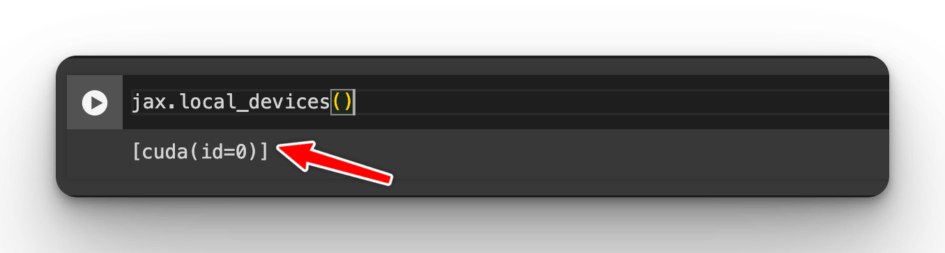
Create TensorFlow Dataset
JAX doesn't ship with any data loading functionality. You can use your favorite library to load and process the data. In this case, let's use TensorFlow. First, define the path to the images and the batch size:
base_dir = "dog vs cat/dataset/training_set"
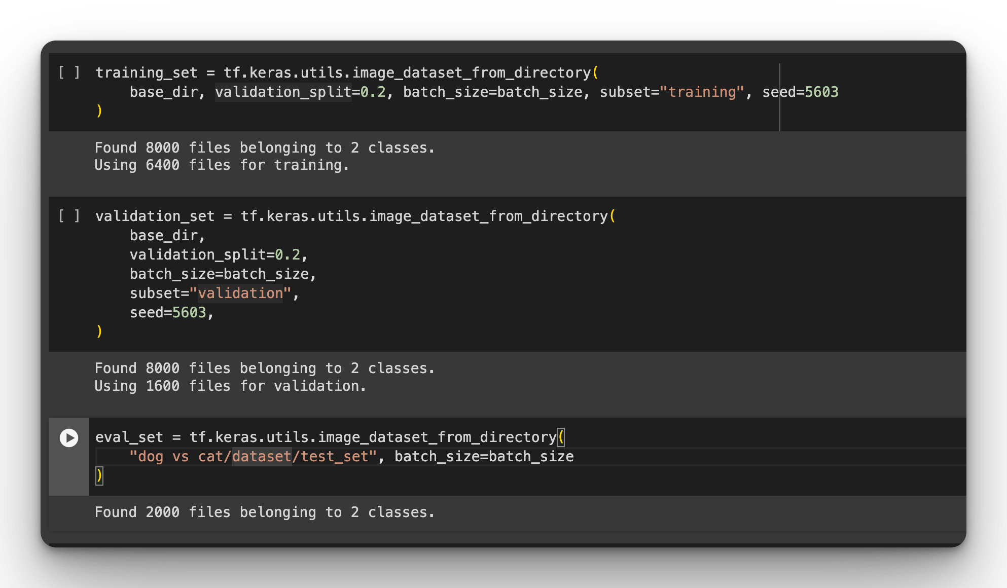
batch_size = 64Load the training, testing, and validation images from the folder:
training_set = tf.keras.utils.image_dataset_from_directory(
    base_dir, validation_split=0.2, batch_size=batch_size, subset="training", seed=5603
)

validation_set = tf.keras.utils.image_dataset_from_directory(
    base_dir,validation_split=0.2,batch_size=batch_size,subset="validation",seed=5603,
)

eval_set = tf.keras.utils.image_dataset_from_directory(
    "dog vs cat/dataset/test_set", batch_size=batch_size
)
Scale TensorFlow Dataset
Next, define functions for scaling and resizing the images. Scaling is necessary for stabilizing the training process by creating small numbers. We also resize all the images to be of the same size. The larger the images the longer training will take.
IMG_SIZE = 128

resize_and_rescale = tf.keras.Sequential(
    [
        tf.keras.layers.Resizing(IMG_SIZE, IMG_SIZE),
        tf.keras.layers.Rescaling(1.0 / 255),
    ]
)
How to Perform Image Augmentation in JAX
Data augmentation modifies existing data to prevent the model from overfitting by passing images of different aspects to the model. In JAX we can do this using the PIX library. In this case, we apply the following transformations:
- Brightness adjustment
- Flipping the images
- Rotating the images
Here's the function that will do that:
rng = jax.random.PRNGKey(0)
rng, inp_rng, init_rng = jax.random.split(rng, 3)

delta = 0.42
factor = 0.42

@jax.jit
def data_augmentation(image):
    new_image = pix.adjust_brightness(image=image, delta=delta)
    new_image = pix.random_brightness(image=new_image, max_delta=delta, key=inp_rng)
    new_image = pix.flip_up_down(image=image)
    new_image = pix.flip_left_right(image=new_image)
    new_image = pix.rot90(k=1, image=new_image) # k = number of times the rotation is applied

    return new_image
On line 2 above, we create a key and pass it on line 10 since the process is random. This is important in ensuring that we get the same transformation whenever the process is called using the same key. This is in line with JAX's expectation of pure functions.
Visualize Augmented Images in JAX
Apply the function to a bunch of images and visualize them using Matplotlib to ensure that everything is working as expected.
plt.figure(figsize=(10, 10))
augmented_images = []
for images, _ in training_set.take(1):
  for i in range(9):
    augmented_image = data_augmentation(np.array(images[i], dtype=jnp.float32))
    augmented_images.append(augmented_image)
    ax = plt.subplot(3, 3, i + 1)
    plt.imshow(augmented_images[i].astype("uint8"))
    plt.axis("off")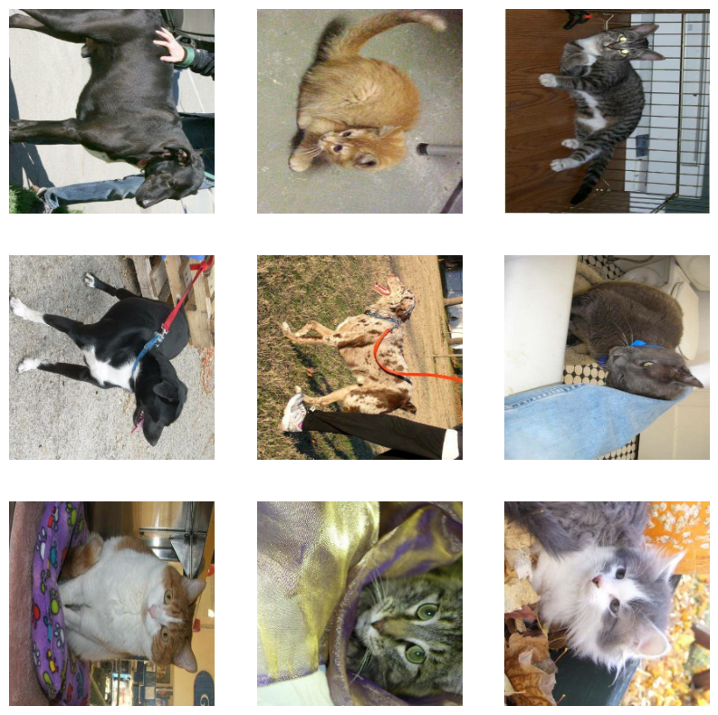
mlnuggets newsletter
Join the newsletter to receive the technical deep dives in your inbox.
Create VMAP Dataset
When creating the augmented images above, we used a for loop. However, we don't want to do this when training the model because it's inefficient. The solution is to use a mapping function that will do this automatically. Fortunately JAX, ships with the vmap function that enables you to easily convert a function designed for a single example to run in a batch.
jit_data_augmentation = jax.vmap(data_augmentation)Convert Dataset to NumPy Arrays
The resulting data will be TensorFlow tensors because we used TensorFlow to process the data. However, passing TensorFlow tensors to a JAX model will lead to data type errors. We, therefore, have to convert the image data to NumPy arrays.
Start by shuffling the dataset and applying the scale and resizing functions.
AUTOTUNE = tf.data.AUTOTUNE


def prepare(ds, shuffle=False):
    # Rescale and resize all datasets.
    ds = ds.map(lambda x, y: (resize_and_rescale(x), y), num_parallel_calls=AUTOTUNE)

    if shuffle:
        ds = ds.shuffle(1000)

    # Use buffered prefetching on all datasets.
    return ds.prefetch(buffer_size=AUTOTUNE)


train_ds = prepare(training_set, shuffle=True)
val_ds = prepare(validation_set)
evaluation_set = prepare(eval_set)
Next, convert the datasets into NumPy arrays using TensorFlow datasets:
def get_batches(ds):
    data = ds.prefetch(1)
    # tfds.dataset_as_numpy converts the tf.data.Dataset into an iterable of NumPy arrays
    return tfds.as_numpy(data)

training_data = get_batches(train_ds)
validation_data = get_batches(val_ds)
evaluation_data = get_batches(evaluation_set)
Create CNN in JAX
Defining a CNN in JAX can be done using the setup or compact way. Here's a CNN network with 3 convolutional blocks:
class_names = training_set.class_names
num_classes = len(class_names)

class CNN(nn.Module):
    @nn.compact
    def __call__(self, x):
        x = nn.Conv(features=128, kernel_size=(3, 3))(x)
        x = nn.relu(x)
        x = nn.max_pool(x, window_shape=(2, 2), strides=(2, 2))
        x = nn.Conv(features=64, kernel_size=(3, 3))(x)
        x = nn.relu(x)
        x = nn.max_pool(x, window_shape=(2, 2), strides=(2, 2))
        x = nn.Conv(features=32, kernel_size=(3, 3))(x)
        x = nn.relu(x)
        x = nn.max_pool(x, window_shape=(2, 2), strides=(2, 2))
        x = x.reshape((x.shape[0], -1))  # flatten
        x = nn.Dense(features=256)(x)
        x = nn.Dense(features=128)(x)
        x = nn.relu(x)
        x = nn.Dense(features=num_classes)(x)
        return x
Each CNN block has a different number of features but they all have the same kernel size, window shape, and pooling strides. The convolutional layers are responsible for reducing the size of the image resulting in a feature map. This is done by passing the image through a kernel, usually a 3 by 3 matrix. The size of the feature map is the same as the size of the image because the padding argument is SAME by default. No padding is applied with the VALID option.
The ReLU activation is applied to ensure non-linearity in the network.
Pooling reduces the size of the feature map further by applying a pooling filter, usually a 2 by 2 matrix. Max pooling picks the largest value in each box while pooled computes the mean of the values in a certain box.
We flatted the pooled feature map before passing it to the fully connected layers. This results in a single column known as a flattened feature map.
Initialize JAX CNN Model
Initialize the JAX CNN model with a data sample that is the same shape as the expected image dataset to create the model parameters. The initialization process requires a pseudo-random number (PRNG) key.
model = CNN()
inp = jnp.ones([1, IMG_SIZE, IMG_SIZE, 3])
# Initialize the model
params = model.init(init_rng, inp)
# print(params)
The structure of the parameters is the same as the CNN network you defined. The kernel part indicates the weights and biases of the JAX CNN model. Apply the model to a sample input and check the output:
model.apply(params, inp)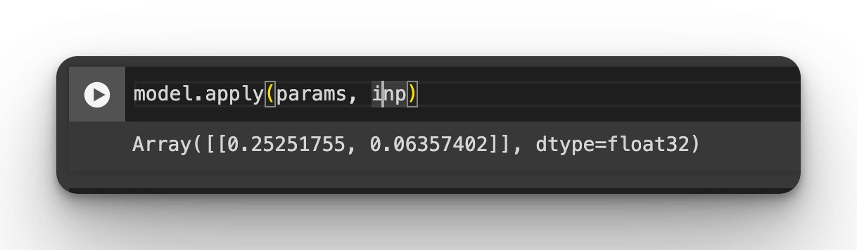
Define Training State for JAX CNN Model
In Flax, the training state is responsible for holding the model variables such as parameters and optimizer state. This is done by subclassing flax.training.train_state. We define a training state with the Adam optimizer at a learning rate of 1e-5.
learning_rate = 1e-5
optimizer = optax.adam(
    learning_rate=learning_rate
)  # lr 1e-4. try 0.001 the default in tf.keras.optimizers.Adam
model_state = train_state.TrainState.create(
    apply_fn=model.apply, params=params, tx=optimizer
)
Compute JAX Metrics
As the model trains, we need to track the loss and accuracy. Later, we can use this to plot the model's performance. Note that on line 3, we apply the jitted and vmaped augmentation function.
We obtain the metrics by:
- Compute the logits by applying the
paramsand images - One hot encoding of the labels
- Computing the loss using
sigmoid_binary_cross_entropyit is since it is a binary classification problem - Obtain the accuracy from the logits
def calculate_loss_acc(state, params, batch):
    data_input, labels = batch
    data_input = jit_data_augmentation(data_input)
    # Obtain the logits and predictions of the model for the input data
    logits = state.apply_fn(params, data_input)
    # Calculate the loss and accuracy
    labels_onehot = jax.nn.one_hot(labels, num_classes=num_classes)
    #uncomment the line below for multiclass classification
    # loss = optax.softmax_cross_entropy(logits, labels_onehot).mean()
    loss = optax.sigmoid_binary_cross_entropy(logits, labels_onehot).mean()
    # comment the line above for multiclass problems
    acc = jnp.mean(jnp.argmax(logits, -1) == labels)
    return loss, acc
Let's break down the code:
data_input, labels = batch: The function expects abatchparameter containing the images and labels.data_input = jit_data_augmentation(data_input): The input data is passed through a function calledjit_data_augmentationthat applies some data augmentation techniques to enhance the diversity of the training data.logits = state.apply_fn(params, data_input): The model's forward pass is computed using theapply_fnmethod of thestateobject. Theparamsare the model parameters anddata_inputthe augmented input data. The resultlogits, represents the raw output of the model before applying any activation function.labels_onehot = jax.nn.one_hot(labels, num_classes=num_classes): The labels are converted into one-hot encoded format using theone_hotfunction from JAX.loss = optax.sigmoid_binary_cross_entropy(logits, labels_onehot).mean(): The loss is computed using the sigmoid binary cross-entropy loss function.acc = jnp.mean(jnp.argmax(logits, -1) == labels): The accuracy is calculated by comparing the predicted class indices (argmax of logits) with the actual labels. The result is a boolean array, andjnp.meanis used to calculate the average accuracy.- The function returns a tuple containing the loss and accuracy.
Test the metrics function on a batch of data:
batch = next(iter(training_data))
calculate_loss_acc(model_state, model_state.params, batch)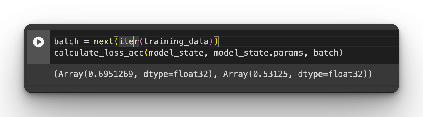
mlnuggets newsletter
Join the newsletter to receive the technical deep dives in your inbox.
Create JAX CNN Training Step
When training the model we need to compute the gradients. This is done using the value_and_grad function. The value part of the name indicates that the function will have additional outputs apart from the gradients. argnums is 1 because the parameters that will be differentiated with respect to are passed as the second argument. Setting has_aux to true means that the second output element is auxiliary data while the first pair is the output of the mathematical function to be differentiated. The apply_gradients function updates the model parameters with the computed gradients. Passing jax.jit to the functions makes them faster since they are optimized for XLA.
@jax.jit  # Jit the function for efficiency
def train_step(state, batch):
    # Gradient function
    grad_fn = jax.value_and_grad(
        calculate_loss_acc,  # Function to calculate the loss
        argnums=1,  # Parameters are second argument of the function
        has_aux=True,  # Function has additional outputs, here accuracy
    )
    # Determine gradients for current model, parameters and batch
    (loss, acc), grads = grad_fn(state, state.params, batch)
    # Perform parameter update with gradients and optimizer
    state = state.apply_gradients(grads=grads)
    # Return state and any other value we might want
    return state, loss, acc
Define JAX Model Evaluation Step
The JAX CNN evaluation step applies the metrics function to the test data and returns the loss and accuracy.
@jax.jit  # Jit the function for efficiency
def eval_step(state, batch):
    # Determine the accuracy
    loss, acc = calculate_loss_acc(state, state.params, batch)
    return loss, acc
Train JAX CNN Model in Flax
Training the JAX CNN model is done in the following steps:
- Apply the
train_stepto the entire training dataset - Obtain the average metrics for each batch
- Compute the mean metrics for each epoch from the batch metrics
- Repeat the same for the evaluation step
- Save the metrics for plotting later
- Print the metrics on the screen
training_accuracy = []
training_loss = []

testing_loss = []
testing_accuracy = []


def train_model(state, train_loader, test_loader, num_epochs=30):
    # Training loop
    for epoch in tqdm(range(num_epochs)):
        train_batch_loss, train_batch_accuracy = [], []
        val_batch_loss, val_batch_accuracy = [], []

        for train_batch in train_loader:
            state, loss, acc = train_step(state, train_batch)
            train_batch_loss.append(loss)
            train_batch_accuracy.append(acc)

        for val_batch in test_loader:
            val_loss, val_acc = eval_step(state, val_batch)

            val_batch_loss.append(val_loss)
            val_batch_accuracy.append(val_acc)

        # Loss for the current epoch
        epoch_train_loss = np.mean(train_batch_loss)
        epoch_val_loss = np.mean(val_batch_loss)

        # Accuracy for the current epoch
        epoch_train_acc = np.mean(train_batch_accuracy)
        epoch_val_acc = np.mean(val_batch_accuracy)

        testing_loss.append(epoch_val_loss)
        testing_accuracy.append(epoch_val_acc)

        training_loss.append(epoch_train_loss)
        training_accuracy.append(epoch_train_acc)

        print(
            f"Epoch: {epoch + 1}, loss: {epoch_train_loss:.2f}, acc: {epoch_train_acc:.2f} val loss: {epoch_val_loss:.2f} val acc {epoch_val_acc:.2f} "
        )

    return state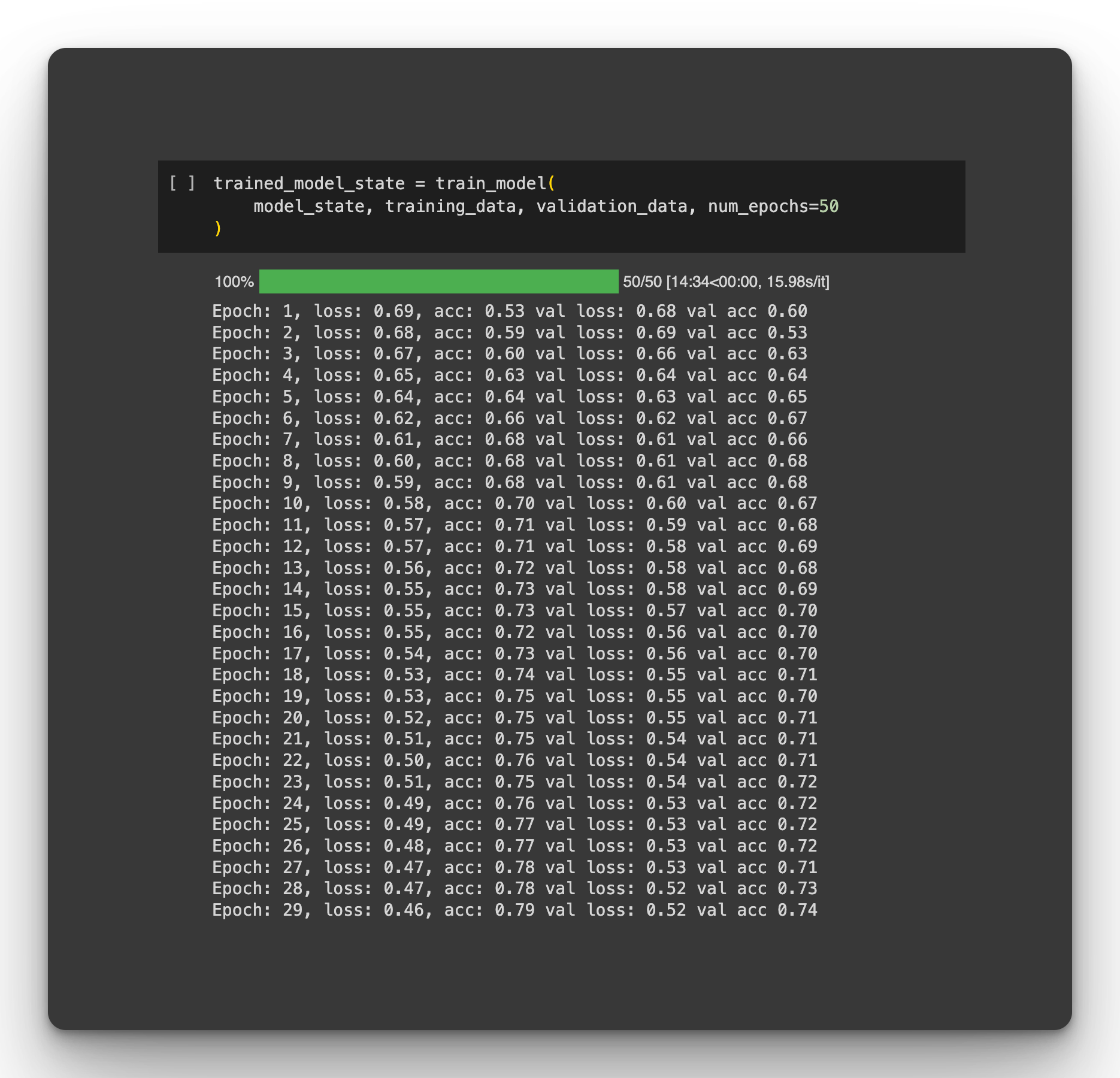
JAX Model Evaluation
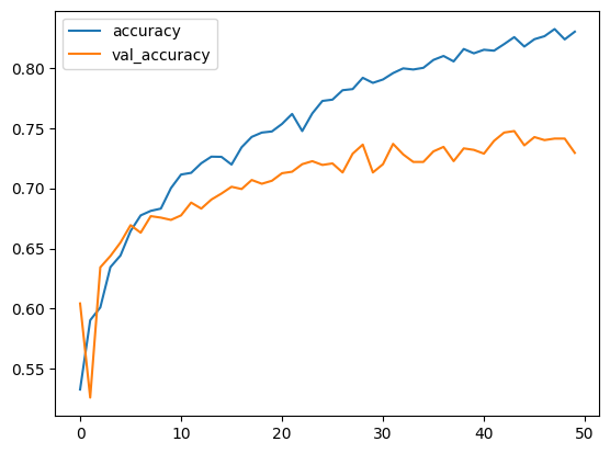
You can save the metrics in a Pandas DataFrame and plot them using Matplotlib.
metrics_df = pd.DataFrame(np.array(training_accuracy), columns=["accuracy"])
metrics_df["val_accuracy"] = np.array(testing_accuracy)
metrics_df["loss"] = np.array(training_loss)
metrics_df["val_loss"] = np.array(testing_loss)
metrics_df[["loss", "val_loss"]].plot()
metrics_df[["accuracy", "val_accuracy"]].plot()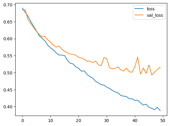
Saving and Loading JAX Models
You may also want to save the trained model for later use. This is done by storing the model checkpoints in a folder:
from flax.training import checkpoints

checkpoints.save_checkpoint(
    ckpt_dir="/content/my_checkpoints/",  # Folder to save checkpoint in
    target=trained_model_state,  # What to save. To only save parameters, use model_state.params
    step=100,  # Training step or other metric to save best model on
    prefix="my_model",  # Checkpoint file name prefix
    overwrite=True,  # Overwrite existing checkpoint files
)
Load the checkpoint:
loaded_model_state = checkpoints.restore_checkpoint(
    ckpt_dir="/content/my_checkpoints/",  # Folder with the checkpoints
    target=model_state,  # (optional) matching object to rebuild state in
    prefix="my_model",  # Checkpoint file name prefix
)
mlnuggets newsletter
Join the newsletter to receive the technical deep dives in your inbox.
Final Remarks
In this article, you have learned how to define and train convolutional neural networks in JAX. You have also covered:
- How to apply data augmentation for computer vision problems in JAX
- Loading image data in JAX
- How to sanity check the augmented images by visualizing them using Matplotlib
- How to take advantage of
jax.jitto make operations faster - Defining a function that runs for a single example and making it run on a batch using
jax.vmap - Defining training loops in JAX
- How to evaluate the performance of CNN models in JAX
..to mention a few.