How to build CNN in TensorFlow(examples, code, and notebooks)

In the artificial neural networks with TensorFlow article, we saw how to build deep learning models with TensorFlow and Keras. We covered various concepts that are foundational in training neural networks with TensorFlow. In that article, we used a Pandas DataFrame to build a classification model in Keras. This article will focus on solving image-related problems with TensorFlow. You will learn how to create image classification models with Keras and TensorFlow. Let's dive in!

What is CNN?

A Convolutional Neural Network(CNN) is a special artificial neural network that processes image data and detects complex features from data. CNNs are primarily used in image tasks and in other problems such as natural language processing tasks.    

How do CNNs work?

The internal working of CNNs is a little different from that of regular artificial neural networks. In this section, let's explore how CNNs work.

Convolution

Image data is usually large. We, therefore, can't pass entire images to a neural network. This because:

• Passing the entire image requires more compute power and processing time.
• The network doesn't require the entire image but only features that are important in identifying the image.

The process of reducing the size of the image is known as convolution. The convolution operation results in a feature map, also known as a convolved feature or activation map. The convolution process works by passing a feature detector over the input image. The feature detector also goes by other names such as kernel or filter.

In most cases, the kernel is a 3 by 3 matrix. However, different kernel sizes can be used. The feature map is obtained through an element-wise multiplication of the kernel with input images and summing the values.

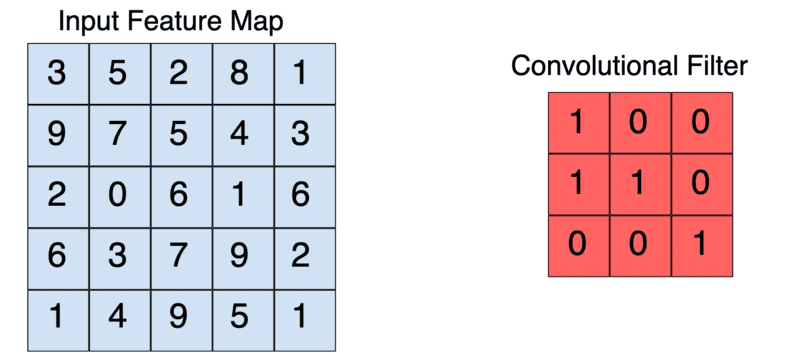
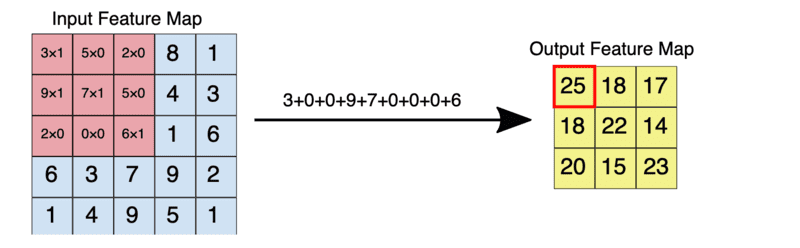
Given the above input image and filter, the convolution operation looks like this:

• 3x1 + 5x0 + 2x0 + 9x1+7x1 + 5x0 + 2x0 + 0x0 + 6x1 =3+0+0+9+7+0+0+6= 25
• Slide the kernel through the entire input image to obtain all the values as we have done above.  

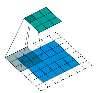
The kernel moves over the input images through steps known as strides. The number of strides is defined while designing the network.  

The size of the feature map is the same as the size of the kernel.

Padding

Applying the kernel reduces the output to the size of the kernel. However, keeping the same image size after applying the kernel might be desirable in specific scenarios. This is important, for instance, when the edges of the images have information that may be critical in classifying the image.

Maintaining the size of the feature map as the input image is achieved via padding. Padding increases the size of the input image by adding zeros around the image such that when the kernel is applied, the output has the same size as the input image. The type of padding is also defined when creating the network. The options are:

• Same to pad such that the size of the input image and the feature map are the same.
• Valid to apply no padding.  

Apply ReLU

The Rectified Linear Unit (ReLU) is applied during the convolution operation to ensure no-linearity. This forces all values below zero to zero while the others are returned as the actual values.  

Pooling

At this point, we have a feature map. It is desirable to reduce the size of the feature map further. This is done via a process known as pooling. Like in the convolution operation, another filter is applied to reduce the size of the feature map. This filter is referred to as a pooling filter. The pooling filter is usually a 2 by 2 matrix. There are various pooling strategies, including:

• Max pooling where the filter slides over the feature map picking the largest value in each box.

• Average pooling that computes the average of the values in a given box.

Pooling results in a pooled feature map.

Dropout regularization

It is usually good practice to drop some connections between layers in CNNs to prevent overfitting. This forces the network to identify essential features needed to identify an image and not memorize the training data.    

Flattening

It's time to pass the pooled feature map to a fully connected layer. However, before we can do that, we have to convert it to a single column. This is done by flattening the pooled feature map. This results in a flattened feature map.  

Full connection

A CNN can have several fully connected layers after the flattening operation. However, the last fully connected layer is responsible for generating the neural network's output.    

Activation function

An activation function is applied on the last fully connected layer depending on the number of categories in the images. The sigmoid activation function is used in a binary problem, while the softmax activation function is applied in a multiclass task.    

Convolutional Neural Networks (CNN) in TensorFlow

With the basics out of the way, let's build CNNs with TensorFlow. First, we need to ensure that TensorFlow is installed.

How to install TensorFlow

TensorFlow is an open-source deep learning framework that enables us to build and train CNNs. TensorFlow can be installed from the Python Index via the pip command. TensorFlow is already installed on Google Colab. You will, therefore, not install it when working in this environment.  

# Requires the latest pip
pip install --upgrade pip

# Current stable release for CPU and GPU
pip install tensorflow

# Or try the preview build (unstable)
pip install tf-nightly

You can also install TensorFlow using Docker. Docker is the easiest way to install TensorFlow on Linux if GPU support is desired.

 docker pull tensorflow/tensorflow:latest  # Download latest stable image
 docker run -it -p 8888:8888 tensorflow/tensorflow:latest-jupyter  # Start Jupyter server 

Follow these instructions to install TensorFlow on Apple Silicon machines. This will enable you to train models with GPUs on Mac.

How to confirm TensorFlow is installed

You can confirm that TensorFlow has been installed by printing the version. If TensorFlow is installed, the version will be printed.

import tensorflow as tf
print(tf.__version__)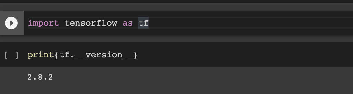

What are Keras and tf.keras?

In TensorFlow 1, Keras and TensorFlow were two separate packages. Keras was being used as the high-level API for TensorFlow. Due to its ease of use and popularity, Keras was included as part of TensorFlow 2. Keras is the official high-level API for building deep learning models in TensorFlow. You'll import it into your programs as tf.keras.  

Develop multilayer CNN models

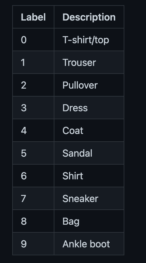
Let's use the Fashion MNIST dataset to illustrate how to build multilayer CNN models with TensorFlow. The dataset contains 60,ooo grayscale images for training and  10,000 for testing. Like the digits MNIST dataset, the image size is 28 by 28.

Data preprocessing

First, load the dataset. We use Layer to achieve this.

# !pip install layer -U # install Layer to load the dataset 
import layer
mnist_train = layer.get_dataset('layer/fashion_mnist/datasets/fashion_mnist_train').to_pandas()
mnist_test = layer.get_dataset('layer/fashion_mnist/datasets/fashion_mnist_test').to_pandas()

We can visualize some samples from this dataset.

mnist_train["images"][17]
mnist_test["images"][23]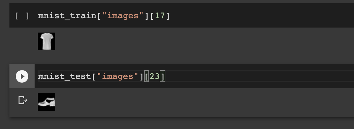

Let's convert these images to NumPy arrays.

import numpy as np
def images_to_np_array(image_column):
    return np.array([np.array(im.getdata()).reshape((im.size[1], im.size[0])) for im in image_column])
train_images = images_to_np_array(mnist_train.images)
test_images = images_to_np_array(mnist_test.images)
train_labels = mnist_train.labels
test_labels = mnist_test.labels

Model definition

Now that the dataset is ready, define the CNN network. The network contains the following layers:

• An input layer with the shape similar to the size of the input image. The last parameter, 1, indicates that the images are grayscale.
• Convolution layer with 32 units, a 3 by 3 kernel size, and a ReLu activation function.
• Pooling layer with a 2 by 2 pooling filter.
• Flatten layer to flatten the pooled feature map.
• Dropout to add dropout regularization to prevent overfitting.
• Fully connected layer–Dense layer– with 10 units representing the number of categories in the dataset and the softmax activation function.

parameters = {"shape":28, "activation": "relu", "classes": 10, "units":12, "optimizer":"adam", "epochs":1,"kernel_size":3,"pool_size":2, "dropout":0.5}
# Setup the layers
model = keras.Sequential(
  [
      keras.Input(shape=(parameters["shape"], parameters["shape"], 1)),
      layers.Conv2D(32, kernel_size=(parameters["kernel_size"], parameters["kernel_size"]), activation=parameters["activation"]),
      layers.MaxPooling2D(pool_size=(parameters["pool_size"], parameters["pool_size"])),
      layers.Conv2D(64, kernel_size=(parameters["kernel_size"], parameters["kernel_size"]), activation=parameters["activation"]),
      layers.MaxPooling2D(pool_size=(parameters["pool_size"], parameters["pool_size"])),
      layers.Flatten(),
      layers.Dropout(parameters["dropout"]),
      layers.Dense(parameters["classes"], activation="softmax"),
  ]
)

Compiling the model

The next step is to compile the neural network. This is where gradient descent is applied. This is the optimization strategy that reduces the errors as the network is learning. There are various optimization strategies but adam is a common approach. It applies the Adam algorithm. In the compile stage, we also define the loss function and the metrics. We use sparse categorical cross-entropy because the labels are integers. The categorical cross-entropy is used when the labels are one-hot encoded.  

# Compile the model
model.compile(optimizer=parameters["optimizer"],
            loss=tf.keras.losses.SparseCategoricalCrossentropy(),
            metrics=['accuracy'])

Train the model

We are ready to train this network using the Fashion MNIST dataset. In TensorFlow, training is done by calling the fit method. Apart from the training and validation data, the fit function expects the number of training iterations– epochs.

history = model.fit(x=train_images, y=train_labels,validation_data=(test_images,test_labels), epochs=parameters["epochs"])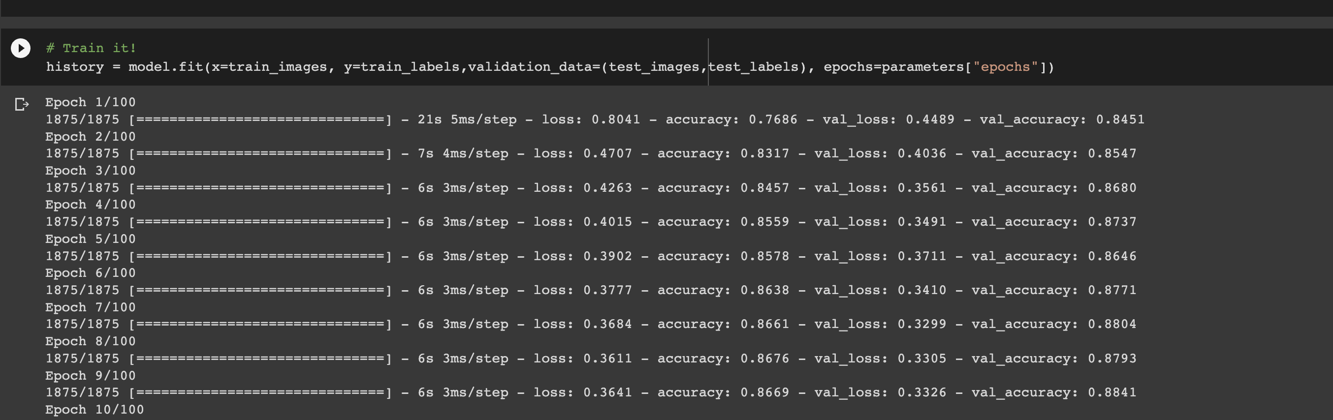

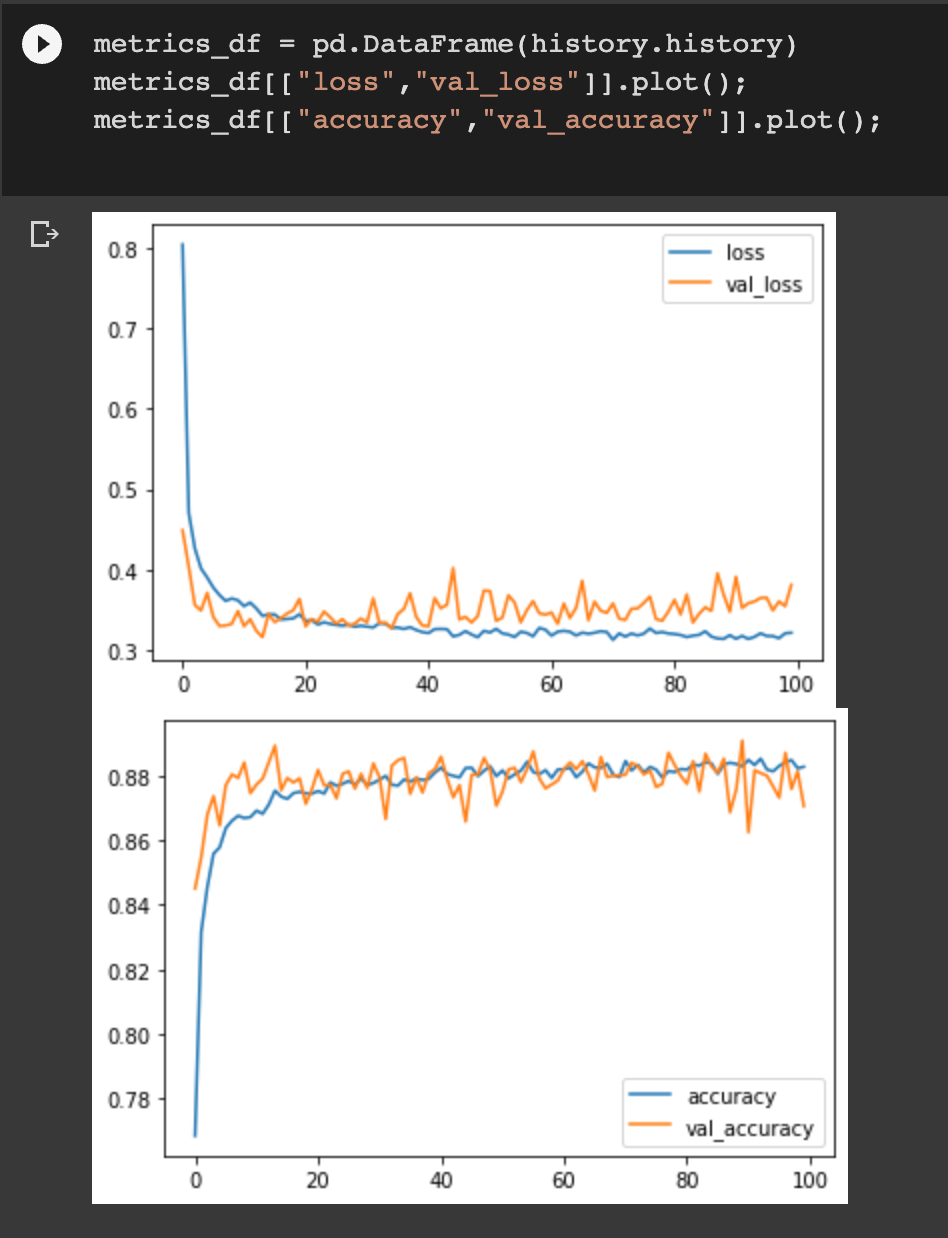
How to plot model learning curves

When training the model, we assigned that process to the history variable. This variable holds the training and validation metrics. We can use that to plot the training and validation metrics.

metrics_df = pd.DataFrame(history.history)
metrics_df[["loss","val_loss"]].plot();
metrics_df[["accuracy","val_accuracy"]].plot();# The semicolon prevents certain matplotlib items from being printed. 

Model evaluation

Let's now evaluate the performance of the network on the testing set. This is done using the evaluate method.    

# And finally evaluate the accuracy
test_loss, test_acc = model.evaluate(test_images,  test_labels, verbose=2)
predictions = model.predict(test_images)
df = pd.DataFrame(predictions, columns=["0","1","2","3","4","5","6","7","8","9"])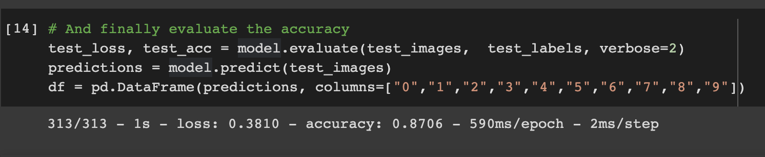

How to halt training at the right time with Early Stopping

CNN models can take a long time to train, especially when the training images are in the thousands. Often, it's good practice to stop training when the network is no longer improving. To achieve this, we apply a built-in function in TensorFlow called EarlyStoppingCallback. The function expects:

• The metrics to monitor.
• The mode, whether to check for the minimum or maximum of the metrics.
• patience to determine how long the network should wait before halting the training if the metric is not improving.

The callback is passed using the callbacks parameter of the fit method.  

callbacks = [tf.keras.callbacks.EarlyStopping(monitor='accuracy', mode="max", patience=3)]
# Compile the model
model.compile(optimizer=parameters["optimizer"],
            loss=tf.keras.losses.SparseCategoricalCrossentropy(),
            metrics=['accuracy'])
history = model.fit(x=train_images, y=train_labels,validation_data=(test_images,test_labels), epochs=parameters["epochs"],callbacks=callbacks)

How to accelerate training with batch normalization

As the name suggests, batch normalization — batchnorm –  involves normalizing the input to the network. Batch normalization ensures that the mean output is close to o and the output standard deviation is close to 1. It normalizes input using the mean and standard deviation of the current training batch. When making predictions, batch normalization normalizes its output using the moving average of the mean and standard deviation of the batches computed during training. Batch normalization is primarily applied in deep neural networks to make training faster.

model = keras.Sequential(
  [
      keras.Input(shape=(parameters["shape"], parameters["shape"], 1)),
      layers.Conv2D(32, kernel_size=(parameters["kernel_size"], parameters["kernel_size"]), activation=parameters["activation"]),
      layers.MaxPooling2D(pool_size=(parameters["pool_size"], parameters["pool_size"])),
      layers.Conv2D(64, kernel_size=(parameters["kernel_size"], parameters["kernel_size"]), activation=parameters["activation"]),
      layers.MaxPooling2D(pool_size=(parameters["pool_size"], parameters["pool_size"])),
      layers.Flatten(),
      layers.Dropout(parameters["dropout"]),
      layers.Dense(64, activation="relu"),
      layers.BatchNormalization(),
      layers.Dense(parameters["classes"], activation="softmax"),
  ]
)
model.compile(optimizer=parameters["optimizer"],
            loss=tf.keras.losses.SparseCategoricalCrossentropy(),
            metrics=['accuracy'])
            
history = model.fit(x=train_images, y=train_labels,validation_data=(test_images,test_labels), epochs=parameters["epochs"])

How to create custom callbacks for TensorFlow CNN

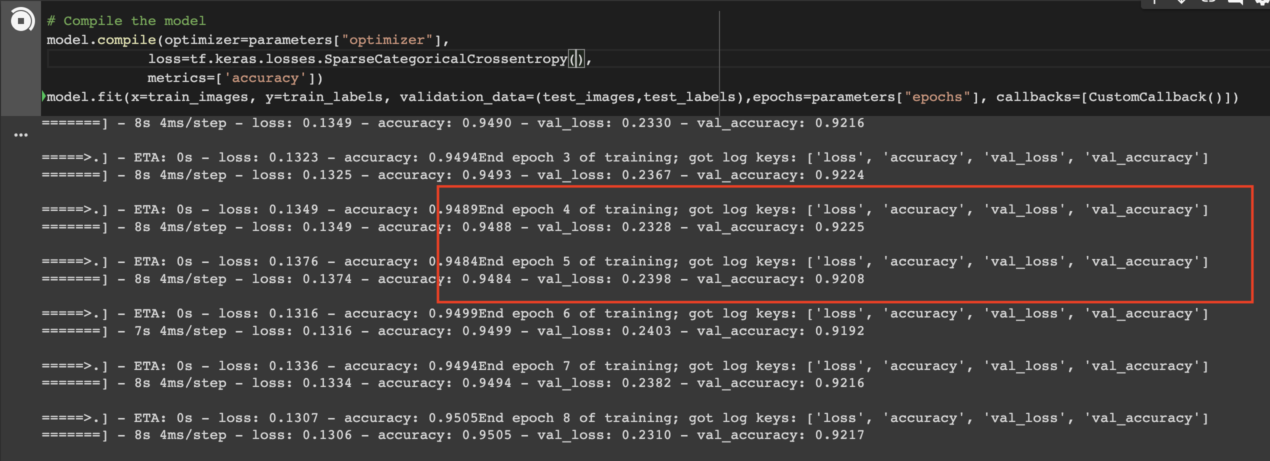
TensorFlow also enables you to define custom callbacks. This is handy when you want to track items not supported by built-in callbacks. The example below prints the keys at the end of every epoch.

from tensorflow.keras.callbacks import Callback 
class CustomCallback(Callback):

    def on_epoch_end(self, epoch, logs=None): 
      keys = list(logs.keys())
      print("End epoch {} of training; got log keys: {}".format(epoch, keys))
# Compile the model
model.compile(optimizer=parameters["optimizer"],
            loss=tf.keras.losses.SparseCategoricalCrossentropy(from_logits=True),
            metrics=['accuracy'])
model.fit(x=train_images, y=train_labels, validation_data=(test_images,test_labels),epochs=parameters["epochs"], callbacks=[CustomCallback()])

How to visualize a deep learning model

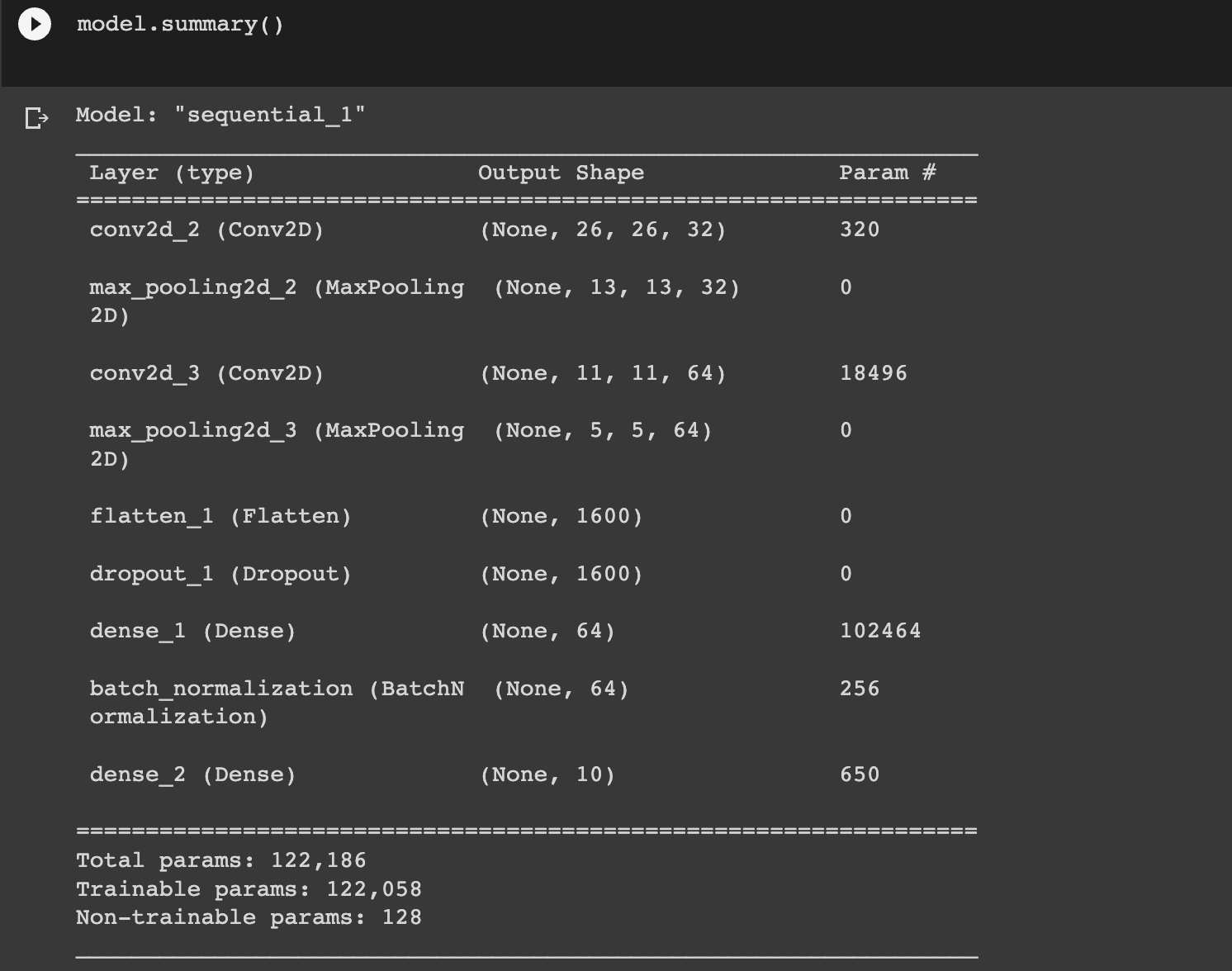
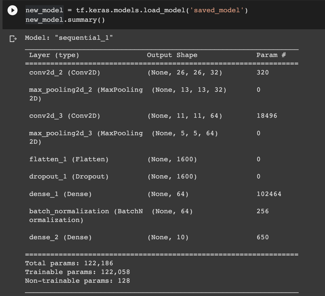
A quick way to visualize a deep learning model is to call the summary function.

model.summary()

On the summary, you will see the following:

• Network layers and their type.
• Output shape for each network.
• Number of parameters for each layer.
• Total number of parameters.
• Total number of trainable and untrainable parameters.

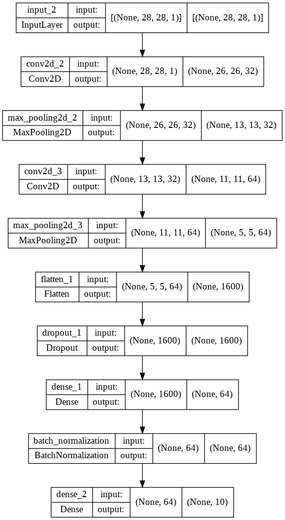
Alternatively, you can also plot the network as an image using the plot_model function.

tf.keras.utils.plot_model(
    model,
    to_file="model.png",
    show_shapes=True,
    show_layer_names=True,
    rankdir="TB",
    expand_nested=True,
    dpi=96,
)

You can follow this plot from the top to see how the shapes change until the last output layer.

How to save and load your model

A deep learning model can be saved and loaded later. For example, you may want to save it and deploy it. TensorFlow enables the saving of a network's weights or the entire model.

model.save_weights('./checkpoints/my_checkpoint')
model.save("saved_model")
new_model = tf.keras.models.load_model('saved_model')
new_model.summary()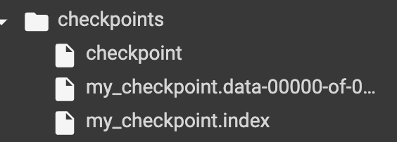

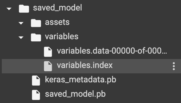
You can then load the model and use it for predictions or re-train it.  

Running CNNs with TensorFlow in the real world

To run CNNs in the real world, we need the ability to load and process image data from a folder. In this part of the article, we'll use the food images dataset available on Kaggle to build an image classification network.  

Loading the images

We start by downloading and extracting the data.

import wget # pip install wget
import tarfile
wget.download("http://data.vision.ee.ethz.ch/cvl/food-101.tar.gz")
food_tar = tarfile.open('food-101.tar.gz')
food_tar.extractall('.') 
food_tar.close()

Generate a tf.data.Dataset

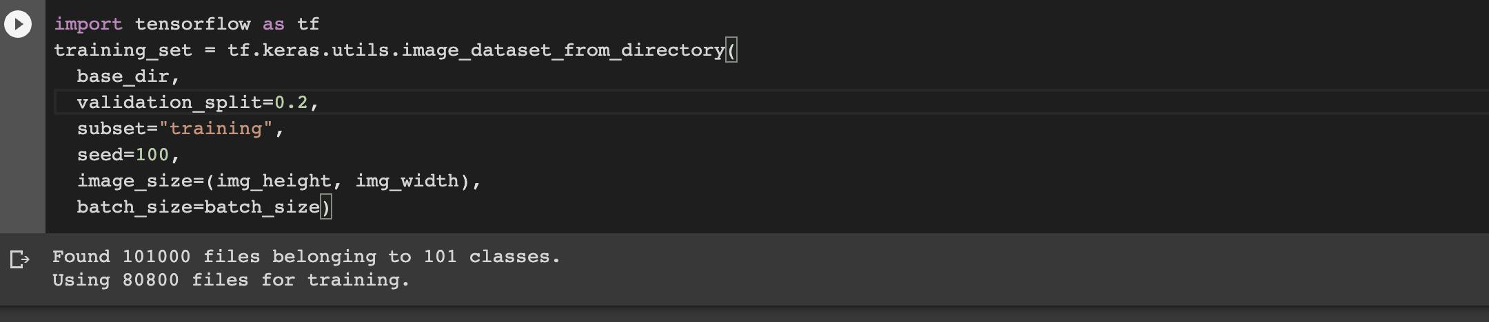
Next, let's load these images using  image_dataset_from_directory from TensorFlow. The function returns a tf.data.Dataset. The function takes the following arguments:

• The directory containing the images.
• The batch size.
• The desired width and height of the images.
• Percentage of the images that should be used for validation declared via the validation_split parameter.
• Whether this will be a training or validation split, in this case, training.  
• label_mode that determines how the labels will be encoded. int encodes them as integers while categorical encodes them as a categorical vector.
• A random seed that controls shuffling and other transformations.

base_dir = 'food-101/images'
batch_size = 32
img_height = 128
img_width = 128
import tensorflow as tf
training_set = tf.keras.utils.image_dataset_from_directory(
  base_dir,
  label_mode="int"
  validation_split=0.2,
  subset="training",
  seed=100,
  image_size=(img_height, img_width),
  batch_size=batch_size)

TensorFlow will infer the labels of the images from the directory structure.  

Next, we do the same to load the validation set.

validation_set = tf.keras.utils.image_dataset_from_directory(
  base_dir,
  validation_split=0.2,
  subset="validation",
  seed=100,
  image_size=(img_height, img_width),
  batch_size=batch_size)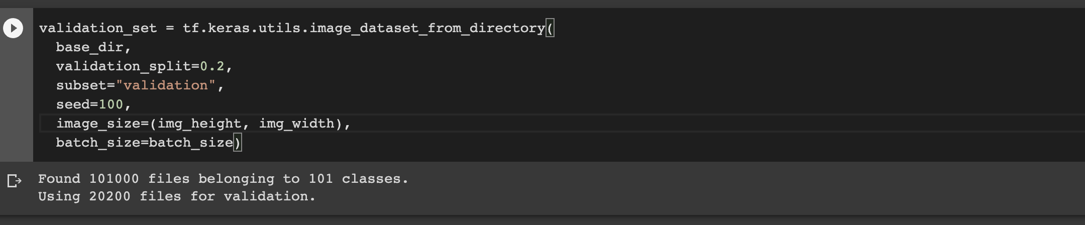

Let's check the class names as inferred by the data loader.

class_names = training_set.class_names
print(class_names)

We can use Matplotlib to visualize a few images.

plt.figure(figsize=(10, 10))
for images, labels in training_set.take(1):
  for i in range(9):
    ax = plt.subplot(3, 3, i + 1)
    plt.imshow(images[i].numpy().astype("uint8"))
    plt.title(class_names[labels[i]])
    plt.axis("off")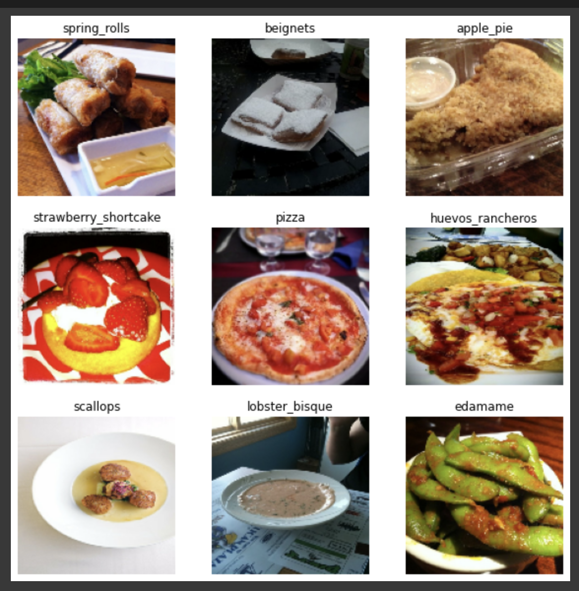

Buffered dataset prefetching

It's important to prefetch data when working with large datasets. Prefetching ensures that the data is available even before it is requested. The number of items to prefetch should be greater than the batch size. You can set this manually or use tf.data.AUTOTUNE to let TensorFlow handle this dynamically.

AUTOTUNE = tf.data.AUTOTUNE

training_ds = training_set.cache().shuffle(1000).prefetch(buffer_size=AUTOTUNE)
validation_ds = validation_set.cache().prefetch(buffer_size=AUTOTUNE)

Image augmentation

Image augmentation involves performing various transformations on training data to ensure that the network sees variations of the same data. Augmentation strategies in image classifications include:

• Flipping the images randomly.
• Random rotations.
• Random zoom.

In general, data augmentation helps to prevent overfitting by exposing the network to images in various aspects.  

from tensorflow import keras
from tensorflow.keras import layers

data_augmentation = keras.Sequential(
  [
    layers.RandomFlip("horizontal",
                      input_shape=(img_height,
                                  img_width,
                                  3)),
    layers.RandomRotation(0.1),
    layers.RandomZoom(0.1),
  ]
)

When defining the network, we will use the above augmentation layer as the first layer in the network. Let's look at what an image would like after the augmentation. We can augment some images and plot them using Matplotlib.

plt.figure(figsize=(10, 10))
for images, _ in training_set.take(1):
  for i in range(9):
    augmented_images = data_augmentation(images)
    ax = plt.subplot(3, 3, i + 1)
    plt.imshow(augmented_images[0].numpy().astype("uint8"))
    plt.axis("off")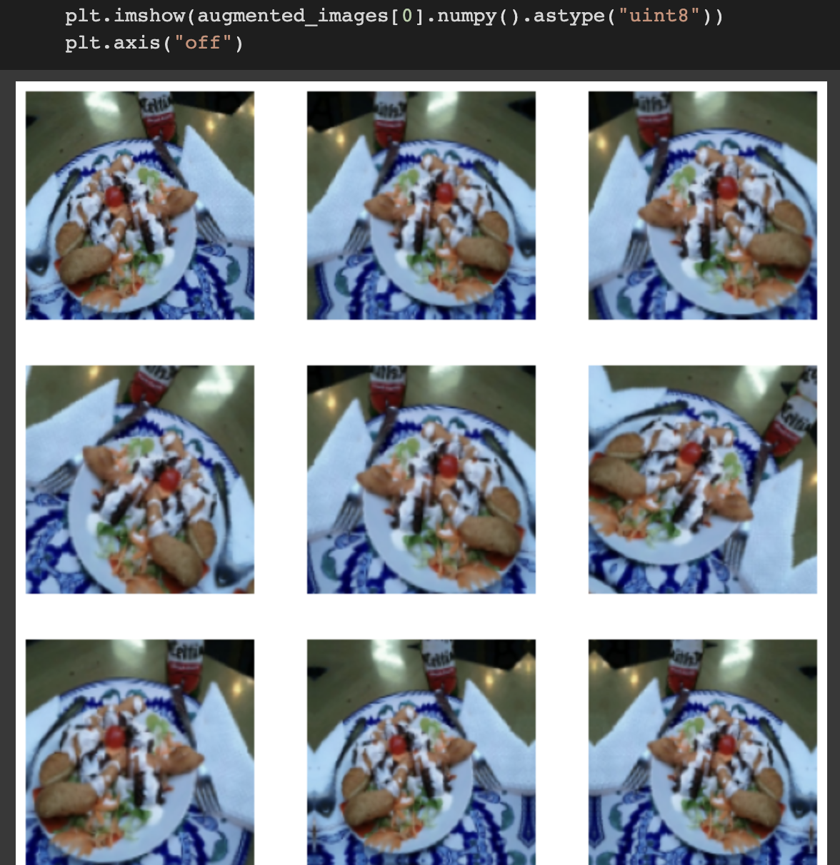

Model definition

We define a neural network with the following layers:

• The image augmentation layer.
• A layer to scale the images.
• A convolution layer with 32 filters, a kernel size of 3 by 3, and the ReLu activation function.  
• A MaxPooling2D layer with a 2 by 2 pool size.
• A dropout layer that "drops" 25% of the connections.
• The Flatten layer and finally
• The final fully connected layer.

model = keras.Sequential([
    data_augmentation,
    layers.Rescaling(1./255),
    layers.Conv2D(filters=32,kernel_size=(3,3),activation='relu'),
    layers.MaxPooling2D(pool_size=(2,2)),

    layers.Conv2D(filters=32,kernel_size=(3,3), activation='relu'),
    layers.MaxPooling2D(pool_size=(2,2)),
    layers.Dropout(0.25),

    layers.Conv2D(filters=64,kernel_size=(3,3), activation='relu'),
    layers.MaxPooling2D(pool_size=(2,2)),
    layers.Dropout(0.25),

    layers.Flatten(),
    layers.Dense(128, activation='relu'),
    layers.Dropout(0.25),
    layers.Dense(len(class_names), activation='softmax')])

Compiling the model

Let's compile the network to prepare it for training.

model.compile(optimizer='adam',
              loss=tf.keras.losses.SparseCategoricalCrossentropy(),
               metrics=['accuracy'])

Training the model

Train the model while applying the Early Stopping callback.

callback = tf.keras.callbacks.EarlyStopping(monitor='loss', patience=3)
epochs=100
history = model.fit(training_set,validation_data=validation_set, epochs=epochs,callbacks=[callback])

Model evaluation

Evaluate the trained model using the evaluate function.

loss, accuracy = model.evaluate(validation_set)
print('Accuracy on test dataset:', accuracy)

Monitoring the model’s performance

Let's visualize the performance of the model using Matplotlib.

import pandas as pd
metrics_df = pd.DataFrame(history.history)
loss, accuracy = model.evaluate(validation_set)
metrics_df[["loss","val_loss"]].plot();
metrics_df[["accuracy","val_accuracy"]].plot();

Visualize CNN graph with TensorBoard

We can visualize the CNN graph using the TensorBoard callback. The TensorBoard callback takes the following parameters:

• The folder where the logs will be saved.
• histogram_freq determines the frequency at which the weight histograms will be computed. This requires validation split or validation data to be provided.
• Setting write_graph to true is what shows the graph of the network.
• write_images as true writes the model weights so that they can be visualized on TensorBoard.
• Setting update_freq as epoch writes the losses and metrics to TensorBoard after each epoch. Writing too often to TensorBoard may slow down the training.

log_folder ="logs"
tensorboard_callback = tf.keras.callbacks.TensorBoard(log_dir=log_folder, 
                                                      histogram_freq=1,
    write_graph=True,
    write_images=True,
    update_freq='epoch'
    )

# Compile the model
model.compile(optimizer='adam',
              loss=tf.keras.losses.SparseCategoricalCrossentropy(),
               metrics=['accuracy'])
model.fit(training_set,validation_data=validation_set,epochs=2, callbacks=[tensorboard_callback])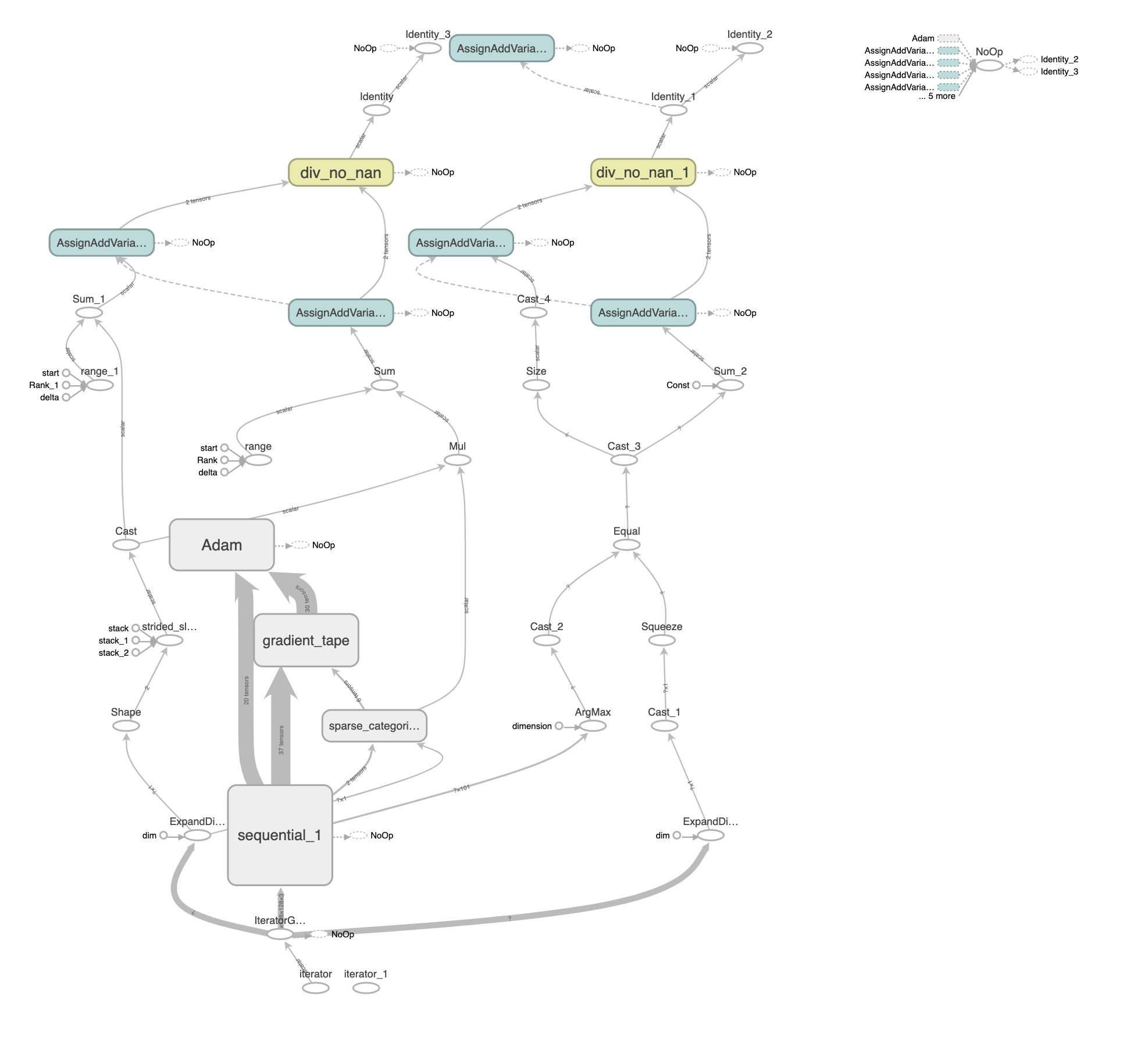

You can also interact with the graph on TensorBoard.

Read more: TensorBoard tutorial (Deep dive with examples and notebook)

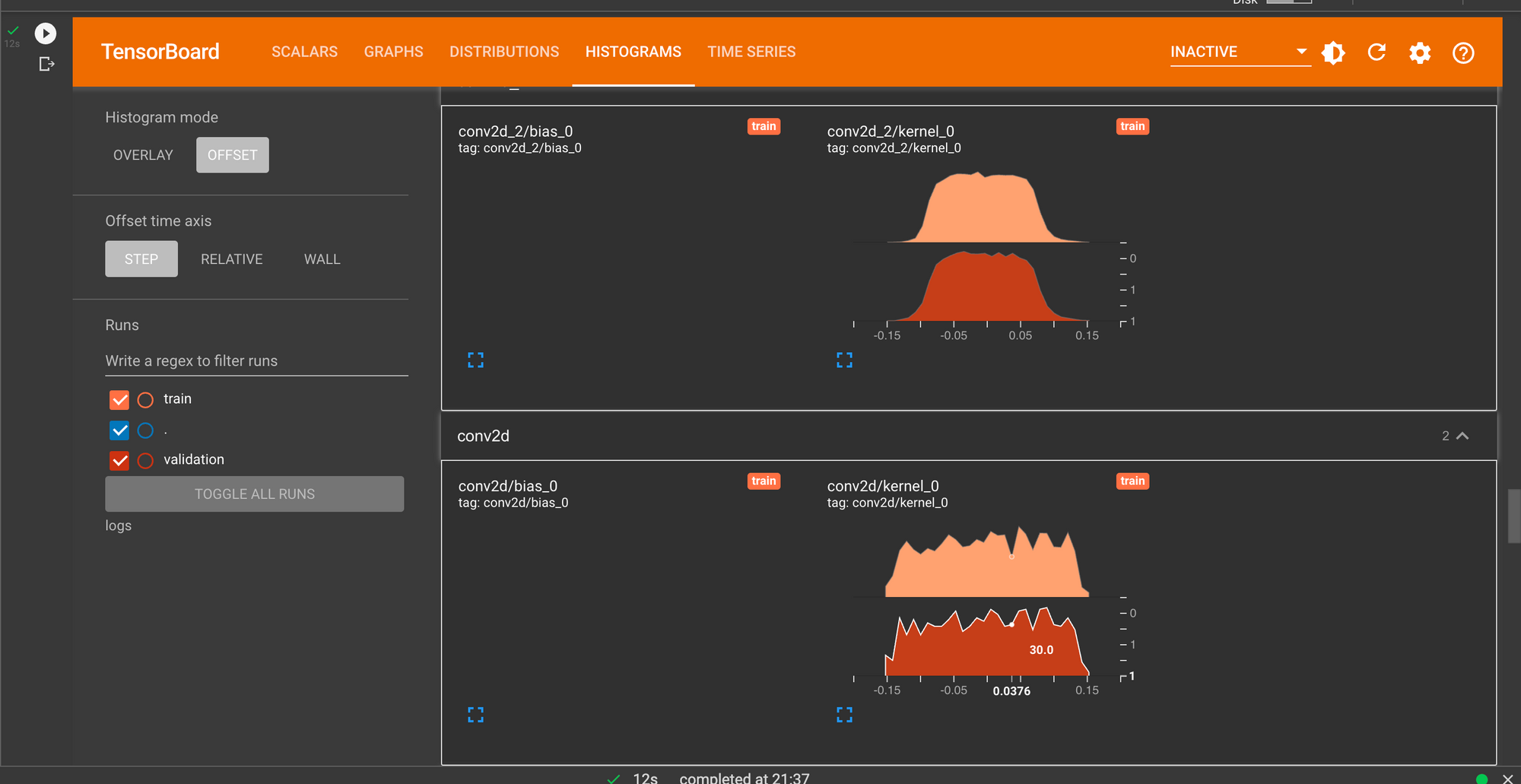
On the Histogram dashboard, we see the weight and biases histogram of the network. Histograms are a great way to visualize the activations of certain layers in the network. You can also use it to check changes in the weights and biases as the network is trained.  

How to profile with TensorBoard

Another thing we can do with TensorBoard is to profile the training of the CNN. This is done by including the profile_batch argument in the TensorBoard callback. In this case, we profile batches 2 to 5. Using the update_freq as 1 means that losses and metrics will be written to TensorBoard at every batch.

Ensure that the profile plugin is installed:

pip install -U tensorboard_plugin_profile

Next, define the TensorBoard callback and pass it to the model training function. Compile and train the network again. Run TensorBoard and select the Profile dashboard to see the profile analysis.  

tensorboard_callback = tf.keras.callbacks.TensorBoard(log_dir=log_folder, profile_batch='2,5', update_freq=1)
# Compile the model
model.compile(optimizer='adam',
              loss=tf.keras.losses.SparseCategoricalCrossentropy(),
               metrics=['accuracy'])
# model.fit(training_set,validation_data=validation_set,epochs=2, callbacks=[tensorboard_callback])
history = model.fit(image_batch, labels_batch,validation_split=0.2, epochs=1,callbacks=[tensorboard_callback])
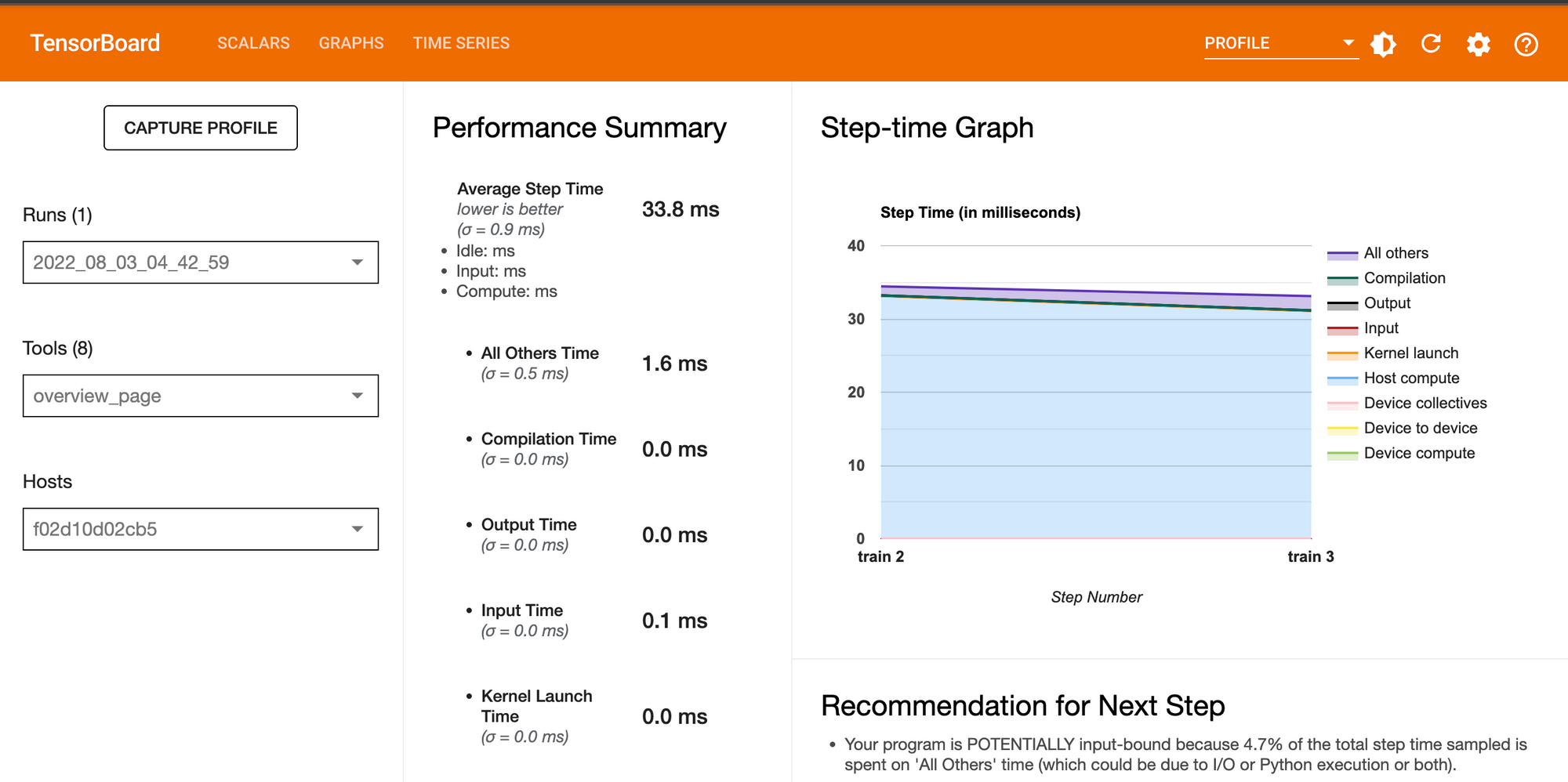
%tensorboard --logdir={log_folder}

On the Overview page, we see the execution summary and some recommendations for improving the model's performance.

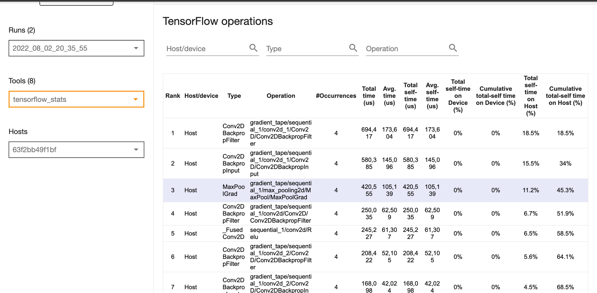
The TensorFlow Stats tool shows the performance of all TensorFlow operations executed during the profiling session.  

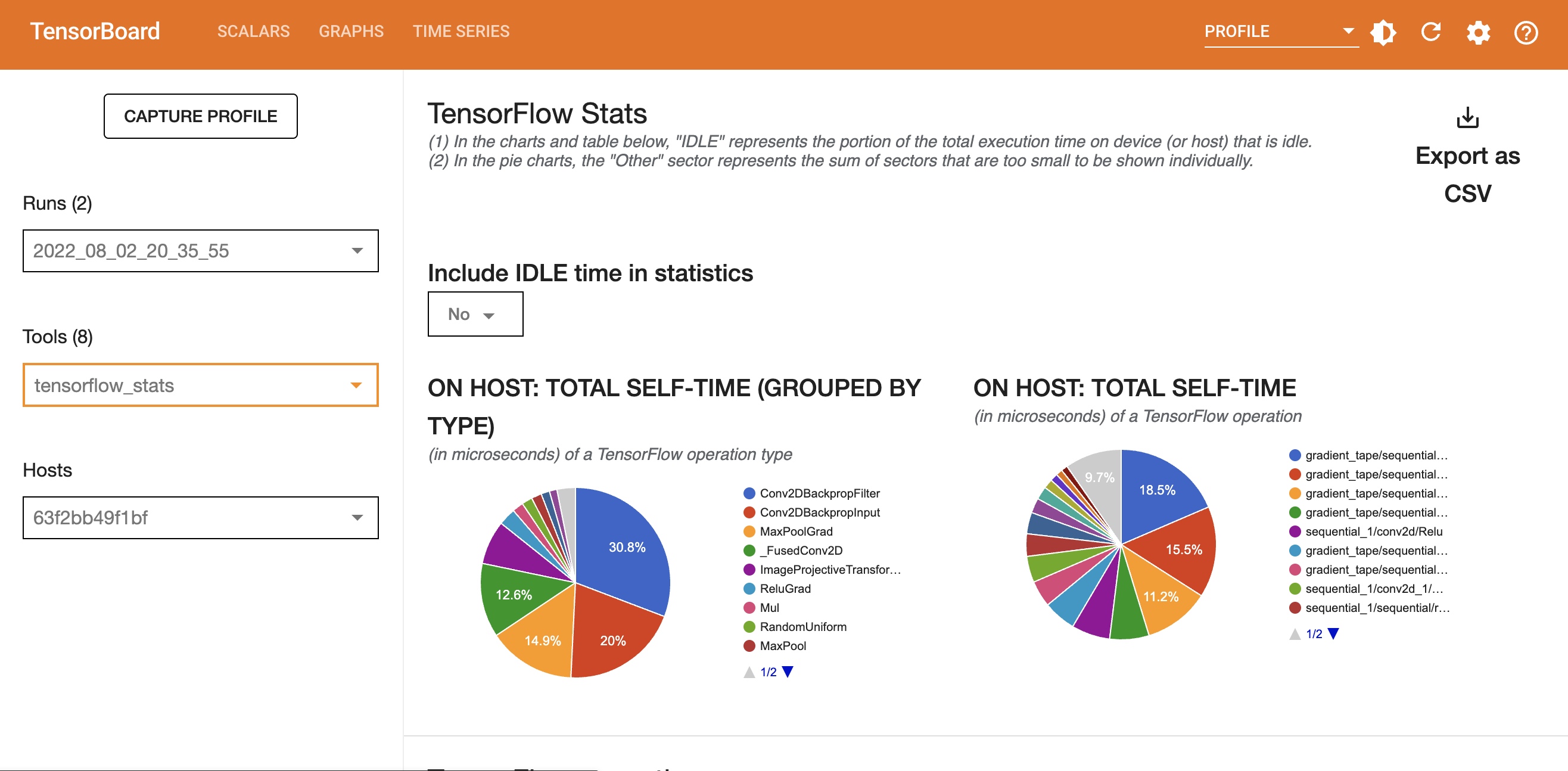
The lower sections of the TensorFlow stats tools show TensorFlow operations. For example, in the image below, we can see familiar items such as Conv2D and MaxPool.

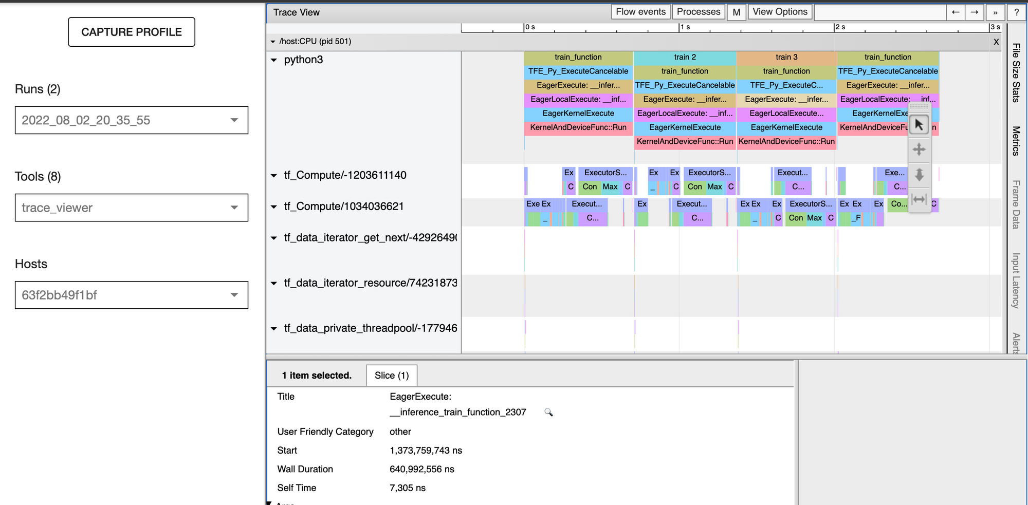
The Trace Viewer under the tools section shows performance bottlenecks in the input pipeline. It shows a timeline of events as they occur in the CPU and GPU. The colored rectangular boxes on the timeline represent individual events. Clicking an event shows more information about it in the section below the Trace Viewer. For example, in the image below, we see the start time and duration of the clicked event.

Making predictions

Let's look at how to use the trained model to make predictions on a new image. We start by loading a new image and adding the batch dimension.

image_url = "https://upload.wikimedia.org/wikipedia/commons/b/b1/Buttermilk_Beignets_%284515741642%29.jpg"
image_path = tf.keras.utils.get_file('Sample_Food', origin=image_url)
test_image = tf.keras.utils.load_img(
    image_path, target_size=(img_height, img_width)
)
img_array = tf.keras.utils.img_to_array(test_image)
img_array = tf.expand_dims(img_array, 0)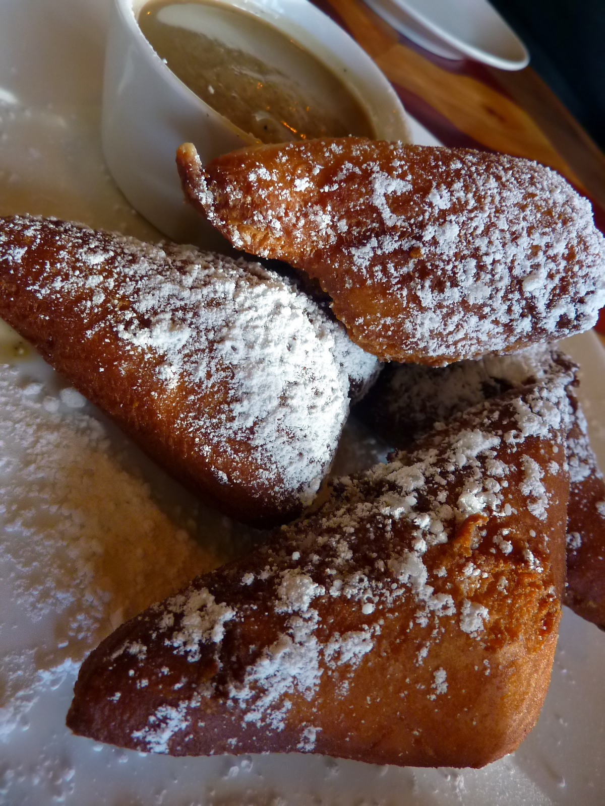 

Next, we scale the image and run predictions on it.

img_array = img_array / 255.0
prediction = model.predict(img_array)
prediction

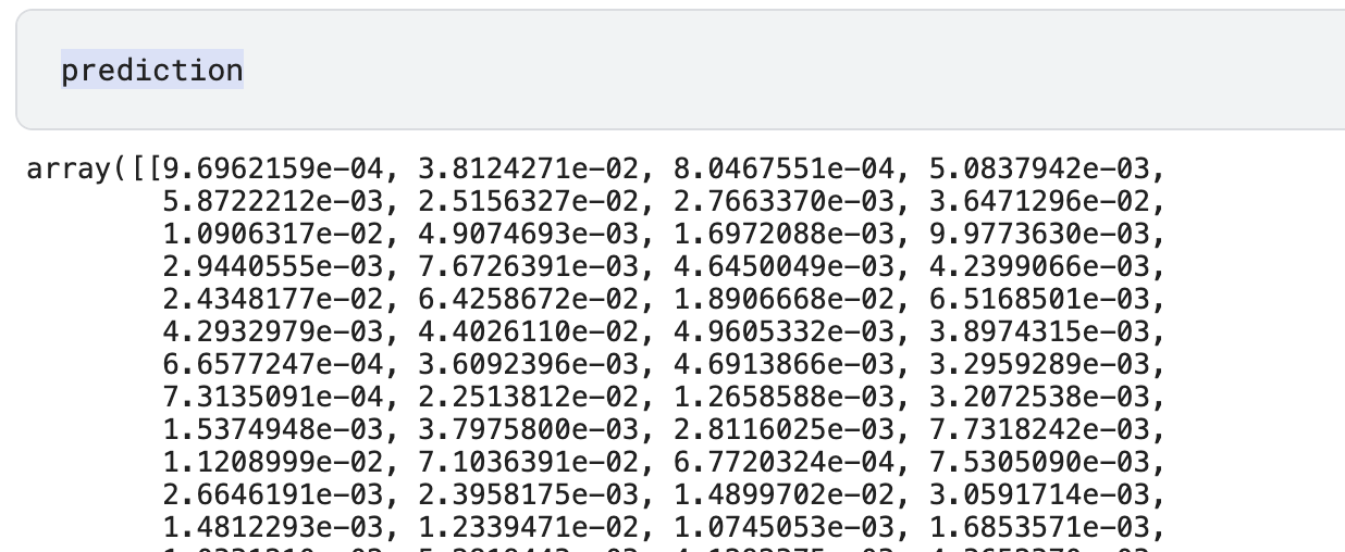
We need to interpret this output to understand the type of food in the image. To do that, we pass the output via the softmax activation function. The addition of all outputs by the softmax function sums to 1.

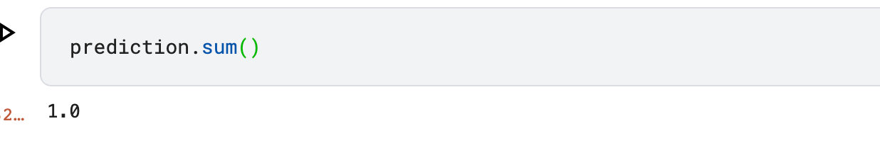
The network outputs a probability for each of the food categories. We pass this to the softmax function and take the maximum value to determine the category of the food.  

import tensorflow as tf
import numpy as np
scores = tf.nn.softmax(prediction[0])
scores = scores.numpy()
f"{class_names[np.argmax(scores)]} with a { (100 * np.max(scores)).round(2) } percent confidence." 
# 'mussels with a 1.14 percent confidence.'

CNN architectures

So far, we have been designing our own CNN networks. However, we can use various CNN architectures to hasten this process. These networks guarantee better performance for image tasks, especially when you use pre-trained models. The pre-trained networks can be used immediately to run predictions on new images or fine-tuned via transfer learning to be specific to a task.

Popular CNN architectures include:

• Xception
• ResNet50
• InceptionV3
• MobileNetV2
• DenseNet121
• NASNetLarge
• EfficientNetB1

Model without weights

We can load any of the above CNN architectures using Keras applications. Let's look at loading ResNet152 architecture. We pass the weights argument as imagenet to load a network that has been trained on the ImageNet dataset.  

model = tf.keras.applications.ResNet152(
    include_top=True,
    weights="imagenet",
    input_tensor=None,
    input_shape=None,
    pooling=None,
    classes=1000,
    classifier_activation="softmax",
)

We can use this network to run predictions on new images immediately. For instance, let's run prediction on the image we used with the CNN network.

To do that, we ensure that the image size is 224 by 224. This is the image size used to train this ResNet network. We also need to process the image the same way the training images were processed. Each of the Keras applications provides a preprocess_input for doing this.

from tensorflow.keras.applications.resnet import preprocess_input, decode_predictions
test_image = tf.keras.utils.load_img(
    image_path, target_size=(224, 224)
)
img_array = tf.keras.utils.img_to_array(test_image)
img_array = tf.expand_dims(img_array, 0) 
x = preprocess_input(img_array)

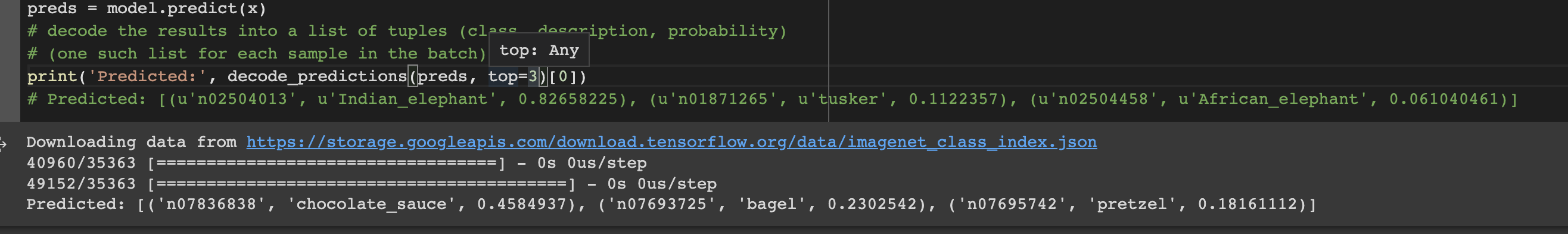
preds = model.predict(x)
# decode the results into a list of tuples (class, description, probability)
# (one such list for each sample in the batch)
print('Predicted:', decode_predictions(preds, top=3)[0])
# Predicted: [('n07836838', 'chocolate_sauce', 0.4584937), ('n07693725', #'bagel', 0.2302542), ('n07695742', 'pretzel', 0.18161112)]

The network has determined the food image to either be a chocolate sauce, bagel or pretzel.  

When loading the ResNet152 network, we included include_top as True. This means that the network will be downloaded with the final fully-connected layer. This is ideal when you want to use the network to make predictions immediately. However, when you want to fine-tune the network on custom data, you set this to false and then include another final fully-connected layer that is specific to your task.  

Model with weights

You may also want to load the CNN architecture without the weights. Doing this means that you will start the training from scratch. In most cases, you'll want to load the networks with the weights to take advantage of the training that has already been done.

model = tf.keras.applications.ResNet152(
    include_top=True,
    weights="imagenet",
    input_tensor=None,
    input_shape=None,
    pooling=None,
    classes=1000,
    classifier_activation="softmax",
)

Final thoughts

We have seen how to build Convolutional Neural Networks with Keras and TensorFlow. We have also covered:

• The steps of training a CNN.
• Adding dropout regularization in CNNs.
• Using batch normalization to speed up training.
• Applying early stopping to train the network for fewer epochs.
• Plotting the learning curves of CNNs.
• Visualizing the graph and histogram of CNN in TensorBoard.
• How to profile the training of the CNN with TensorBoard.
• Data augmentation strategies for image tasks.

...among other topics.

TensorFlow resources

Object detection with TensorFlow 2 Object detection API

How to create custom training loops in Keras

How to train deep learning models on Apple Silicon GPU

How to build artificial neural networks with Keras and TensorFlow

The Complete Data Science and Machine Learning Bootcamp on Udemy is a great next step if you want to keep exploring the data science and machine learning field.

Follow us on LinkedIn, Twitter, GitHub, and subscribe to our blog, so you don't miss a new issue.