
How to build artificial neural networks with Keras and TensorFlow


Building artificial neural networks with TensorFlow and Keras requires understanding some key concepts. After learning these concepts, you'll install TensorFlow and start designing neural networks. This article will cover the concepts you need to comprehend to build neural networks in TensorFlow and Keras. Without further ado, let's get the ball rolling.
What is deep learning?
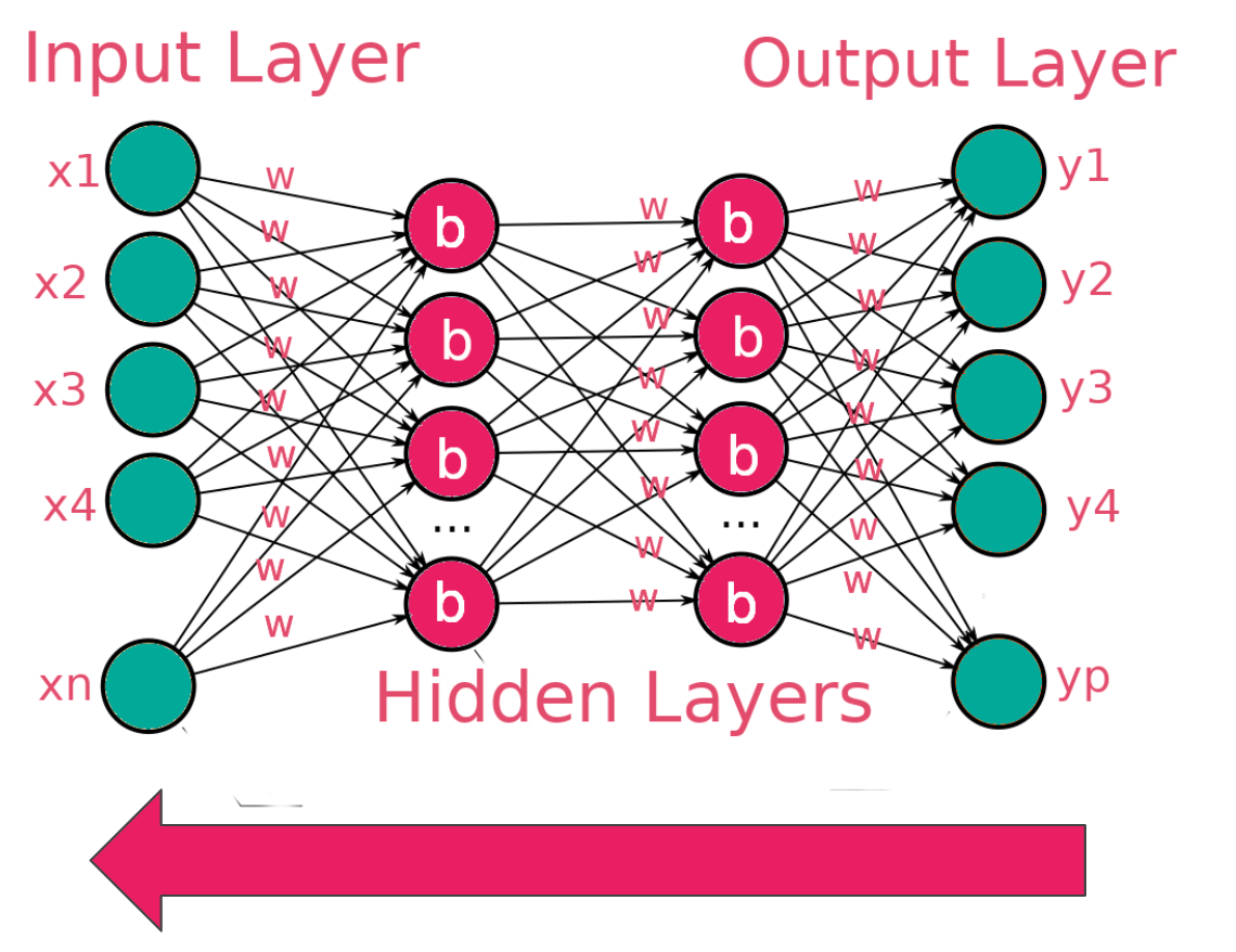
Deep learning is a branch of machine learning that involves building networks that try to mimic the working of the human brain. The dendrite in the human brain represents the input to the network, while the axion terminals represent the output. The cell is where computation would take place before we get the output.

The image below shows a simple network with an input, hidden, and output layer. A network with multiple hidden layers is called a deep neural network.
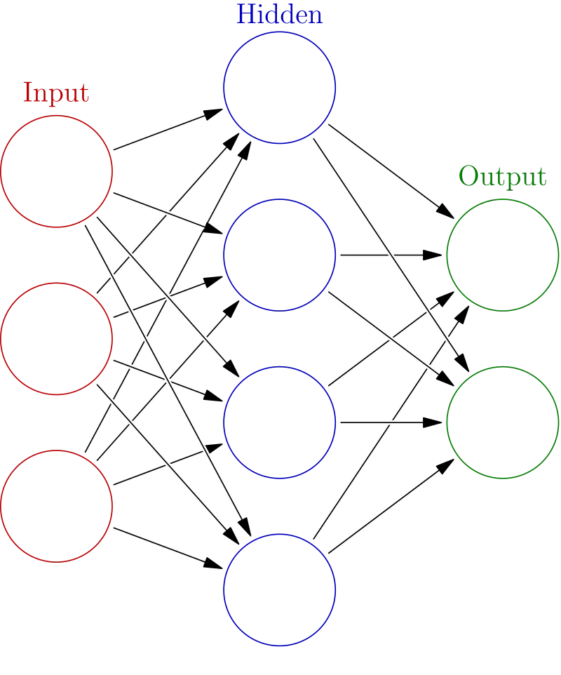
Random weights and biases are initialized when data is passed to a network. Some computation happens in the hidden layers leading to output.

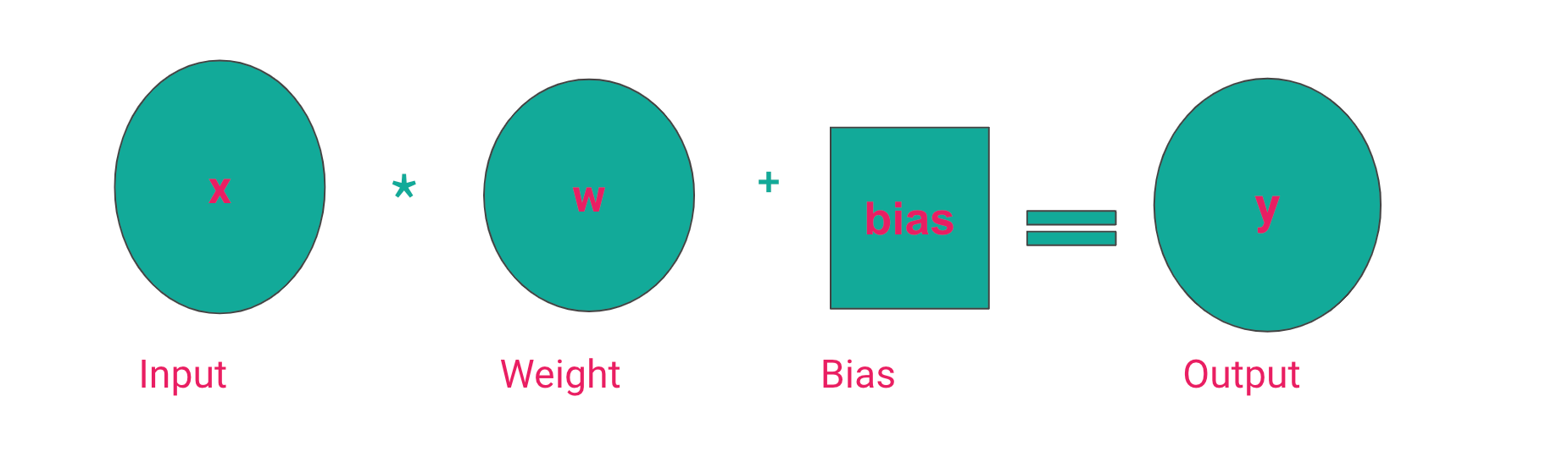
This computation involves multiplying the input by the weights and adding the bias. This is what gives the output. The bias ensures that there is no zero output in case the input and weights are zero.
There are various ways of initializing the weights and biases. The common ones include:
- Initialize with ones.
- Initialize with zeros.
- Use a uniform distribution.
- Apply a normal distribution.
What is an activation function?
The desired output of a neural network depends on the problem being solved. For instance, in a regression problem, the output should be a number predicting the quantity in question. However, in classification problems, it's more desirable to output a probability that is used to determine the category of the prediction. Therefore, to make sure the network outputs the desired results, we pass the computed result through a function that ensures that the result is within a specific range. For example, for probabilities, this number is between 0 and 1. We can't have negative probabilities. The function responsible for capping the result is known as an activation function.
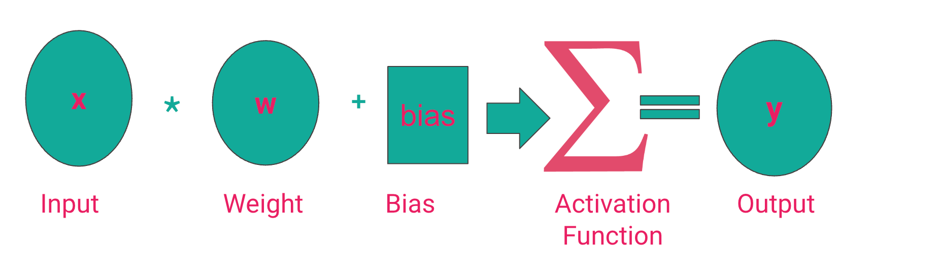
From the above image, we can conclude that the activation function determines the neural network's output. Let's, therefore, mention some of the common activation functions in the deep learning realm.
Sigmoid function
The sigmoid activation function caps output to a number between 0 and 1 and is majorly used for binary classification tasks. Sigmoid is used where the classes are non-exclusive. For example, an image can have a car, a building, a tree, etc. Just because there is a car in the image doesn’t mean a tree can’t be in the picture. Use the sigmoid function when there is more than one correct answer.
Softmax activation function
The softmax activation function is a variant of the sigmoid function used in multi-class problems where labels are mutually exclusive. For example, a picture is either grayscale or color. Use the softmax activation when there is only one correct answer.
Rectified linear unit (ReLU)
The Rectified linear unit (ReLU) activation function limits the output to 0 and above. It is used in the hidden layer of neural networks. It, therefore, ensures no negative outputs from the hidden layers.

How does a neural network learn?
A neural network learns by evaluating predictions against the true values and adjusting the weights. The objective is to obtain the weights that minimize the error, also known as the loss function or cost function. The choice of a loss function, therefore, depends on the problem. Classification tasks require classification loss functions, while regression problems require regression loss functions. As the network learns, the loss functions should decrease.

You might see nans in the loss function while training the network. This means that the network is not learning. In most cases, nans will be developer errors, meaning that there is something you have done or failed to do that is causing the nans. For example:
- The training data contains nans.
- You have not scaled the data.
- Performing operations that lead to nans, for example, division by zero or the square root of a negative number.
- Choosing the wrong optimizer function.
Gradient descent
We have just mentioned that choosing the wrong optimizer could result in nans. So what is an optimizer function? During the training process, errors are reduced by the optimizer function. This optimization is done via gradient descent.
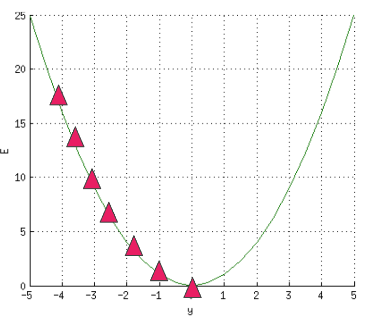
Gradient descent adjusts the errors by reducing the cost function. This is done by computing where the error is at its minimum, commonly known as the local minimum. You can think of this as descending on a slope where the goal is to get to the bottom of the hill, that is, the global minimum. This process involves computing the slope of a specific point on the "hill" via differentiation.
How backpropagation works
The computed errors are passed to the network, and the weights are adjusted. This process is known as backpropagation.
There are several variants of gradient descent. They include:
- Batch Gradient Descent that uses the entire dataset to compute the gradient of the cost function. It is slow since you have to compute the gradient of the entire dataset to perform a single update.
- Stochastic Gradient Descent where the gradient of the cost function is computed from a single training example in every iteration. It is faster.
- Mini-Batch Gradient Descent that uses a sample of the training data to compute the gradient of the cost function.
What is TensorFlow?
TensorFlow is an open-source deep learning framework that enables us to design and train deep learning networks. TensorFlow can be installed from the Python Index via the pip command. TensorFlow is already installed on Google Colab. You will, therefore, not install it when working in this environment.
# Requires the latest pip
pip install --upgrade pip

# Current stable release for CPU and GPU
pip install tensorflow

# Or try the preview build (unstable)
pip install tf-nightly
You can also install TensorFlow using Docker. Docker is the easiest way to install TensorFlow on Linux if GPU support is desired.
 docker pull tensorflow/tensorflow:latest  # Download latest stable image
 docker run -it -p 8888:8888 tensorflow/tensorflow:latest-jupyter  # Start Jupyter server
Follow these instructions to install TensorFlow on Apple arm64 machines. This will enable you to train models with GPUs on Mac.
Why TensorFlow?
There are a couple of reasons why you would choose TensorFlow:
- Has a high-level API that makes it easy to build networks.
- Large ecosystem of tools and libraries.
- Large community that makes it easy to find solutions to common problems.
- Well documented.
- Supports deployment of models on the browser, mobile devices, edge devices, and the cloud.
- Simple and flexible architecture to make research work faster.
TensorFlow vs. Keras
As of TensorFlow 2, Keras is the high-level API for TensorFlow. Keras makes it simple to design and train deep learning networks.
TensorFlow basics
In a moment, we'll be designing neural networks with TensorFlow. However, getting some TensorFlow basics out of the way is essential before we get there.
Tensors
TensorFlow Tensors are multi-dimensional arrays similar to NumPy arrays. Tensors are immutable, meaning they can not be updated once created. Tensors can contain integers, floats, strings, and even complex numbers.
import tensorflow as tf
import numpy as np

x = tf.constant([[7., 8., 9.],[10., 11., 12.]])
print(x)
print(x.shape)
print(x.dtype)
# tf.Tensor(
# [[ 7.  8.  9.]
# [10. 11. 12.]], shape=(2, 3), dtype=float32)
# (2, 3)
# <dtype: 'float32'>
You can perform indexing and operations on Tensors like in NumPy arrays.
x[0]
# <tf.Tensor: shape=(3,), dtype=float32, numpy=array([7., 8., 9.],
# dtype=float32)>
x[1:4]
# <tf.Tensor: shape=(1, 3), dtype=float32, numpy=array([[10., 11., 12.]], # dtype=float32)>
x**2
# <tf.Tensor: shape=(2, 3), dtype=float32, numpy=
# array([[ 49.,  64.,  81.],
#       [100., 121., 144.]], dtype=float32)>
x @ tf.transpose(x) # matrix multiplication
TensorFlow Tensors can also be converted to NumPy arrays.
np.array(x)
x.numpy()
# array([[ 7.,  8.,  9.],
#       [10., 11., 12.]], dtype=float32)
Tensors can contain a different number of elements along a certain axis. These kinds of tensors are known as ragged tensors.
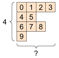
Ragged tensors are created using the tf.ragged.constant function.
try:
  tensor = tf.constant(ragged_list)
except Exception as e:
  print(f"{type(e).__name__}: {e}")
  # ValueError: Can't convert non-rectangular Python sequence to Tensor.
ragged_tensor = tf.ragged.constant(ragged_list)
print(ragged_tensor)
# <tf.RaggedTensor [[0, 1, 2, 3], [4, 5], [6, 7, 8], [9]]>
print(ragged_tensor.shape)
# (4, None)
TensorFlow also supports tensors that have a lot of zeros. These tensors are known as sparse tensors. They can be created using the tf.sparse.SparseTensor function that stores them in a memory-efficient way. For example, converting text data to numerical representation in natural language processing tasks usually results in sparse tensors.
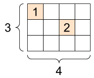
# Sparse tensors store values by index in a memory-efficient manner
sparse_tensor = tf.sparse.SparseTensor(indices=[[0, 0], [1, 2]],
                                       values=[1, 2],
                                       dense_shape=[3, 4])
print(sparse_tensor, "\n")
# SparseTensor(indices=tf.Tensor(
# [[0 0]
# [1 2]], shape=(2, 2), dtype=int64), values=tf.Tensor([1 2], shape=(2,), # dtype=int32), dense_shape=tf.Tensor([3 4], shape=(2,), dtype=int64))
A sparse tensor can also be converted to a dense tensor.
print(tf.sparse.to_dense(sparse_tensor))
# tf.Tensor(
#[[1 0 0 0]
# [0 0 2 0]
#[0 0 0 0]], shape=(3, 4), dtype=int32)
Variables
A TensorFlow variable is used to represent state in TensorFlow programs. Keras stores model parameters in a TensorFlow variable. A TensorFlow variable is also a tensor. A variable is created using tf.Variable.
my_tensor = tf.constant([[8.0, 8.0], [6.0, 5.0]])
my_variable = tf.Variable(my_tensor)
my_variable
# <tf.Variable 'Variable:0' shape=(2, 2) dtype=float32, numpy=
# array([[8., 8.],
#      [6., 5.]], dtype=float32)>
We can check the type and shape of the TensorFlow variable because it's a tensor. It can also be converted to a NumPy array. Tensor operations can also be performed on variables, except that variables can not be reshaped. By default, TensorFlow places variables in the GPU to improve performance. You can, however, override this.
print("Shape: ", my_variable.shape)
print("DType: ", my_variable.dtype)
print("As NumPy: ", my_variable.numpy())
# Shape:  (2, 2)
# DType:  <dtype: 'float32'>
# As NumPy:  [[8. 8.]
# [6. 5.]]
Automatic differentiation
Automatic differentiation is applied at the backpropagation stage of training neural networks. Automatic differentiation in TensorFlow is done using tf.GradientTape. Inputs to this function are usually tf.variables.
x = tf.Variable(47.0)
with tf.GradientTape() as tape:
  y = x**2
# dy = 2x * dx
dy_dx = tape.gradient(y, x)
dy_dx.numpy()
# 94.0
You can use GradientTape to define custom training functions. The GradientTape
will track all trainable variables automatically. tf.gradients computes the gradients with respect to the weights and biases.
# Given a callable model, inputs, outputs, and a learning rate...
def train(model, x, y, learning_rate):

  with tf.GradientTape() as t:
    # Trainable variables are automatically tracked by GradientTape
    current_loss = loss(y, model(x))

  # Use GradientTape to calculate the gradients with respect to W and b
  dw, db = t.gradients(current_loss, [model.w, model.b])

  # Subtract the gradient scaled by the learning rate
  model.w.assign_sub(learning_rate * dw)
  model.b.assign_sub(learning_rate * db)
How TensorFlow works
When TensorFlow is executed eagerly, operations are done in Python, and the results are sent back to Python. The alternative is graph execution, where the operations are executed as a TensorFlow Graph. A Graph represents a data structure representing a set of operations.
The fact that graphs are data structures makes it possible to save and restore them without the original Python code. As a result, these graphs can be used in non-Python environments such as mobile devices, servers, edge devices, and embedded devices. Saved models in TensorFlow are exported as graphs. Graphs enable TensorFlow to run on multiple devices, run in parallel and be fast.
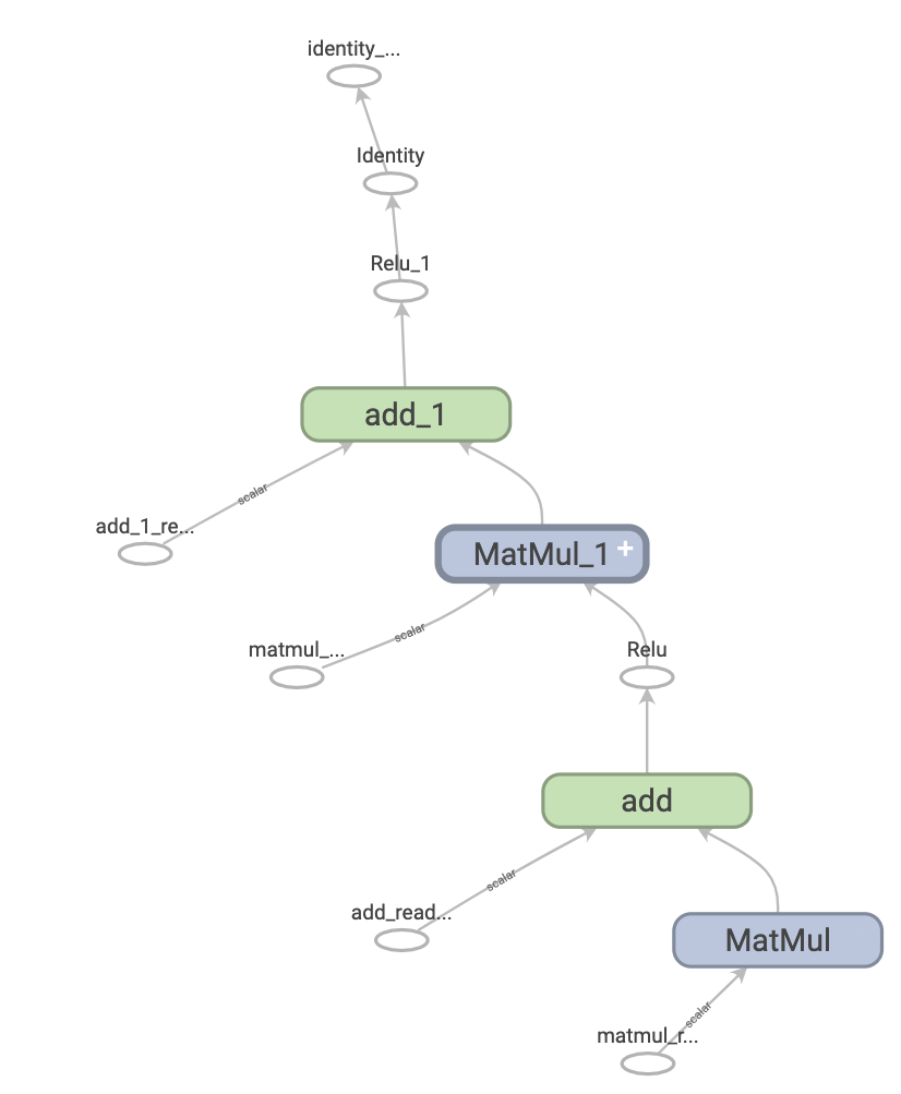
Creating a TensorFlow graph is done via tf.function. It expects a normal function and returns a callable function which creates the TensorFlow graph from the Python function.
def simple_relu(x):
  if tf.greater(x, 0):
    return x
  else:
    return 0

# `tf_simple_relu` is a TensorFlow `Function` that wraps `simple_relu`.
tf_simple_relu = tf.function(simple_relu)

print("First branch, with graph:", tf_simple_relu(tf.constant(1)).numpy())
print("Second branch, with graph:", tf_simple_relu(tf.constant(-1)).numpy())
# First branch, with graph: 1
# Second branch, with graph: 0
How TensorFlow models are defined
A TensorFlow model is made up of layers. Certain mathematical computations occur in the layers. Layers have trainable variables, meaning that these variables are updated as the network is fitted to the training data. In TensorFlow, layers and models are built by creating a class that inherits tf.Module.
class SimpleModule(tf.Module):
  def __init__(self, name=None):
    super().__init__(name=name)
    self.a_variable = tf.Variable(5.0, name="train_me")
    self.non_trainable_variable = tf.Variable(5.0, trainable=False, name="do_not_train_me")
  def __call__(self, x):
    return self.a_variable * x + self.non_trainable_variable

simple_module = SimpleModule(name="simple")

simple_module(tf.constant(5.0))
# <tf.Tensor: shape=(), dtype=float32, numpy=30.0>
How to train artificial neural networks with Keras
With the basics out of the way, we can now embark on a journey to learn how to design and train artificial neural networks in TensorFlow and Keras. We'll use a dataset from Kaggle to train a classification network. The aim is to predict the satisfaction of an airline passenger. Let's start by printing a sample of this dataset.
import pandas as pd
df = pd.read_csv("train.csv")
df.head()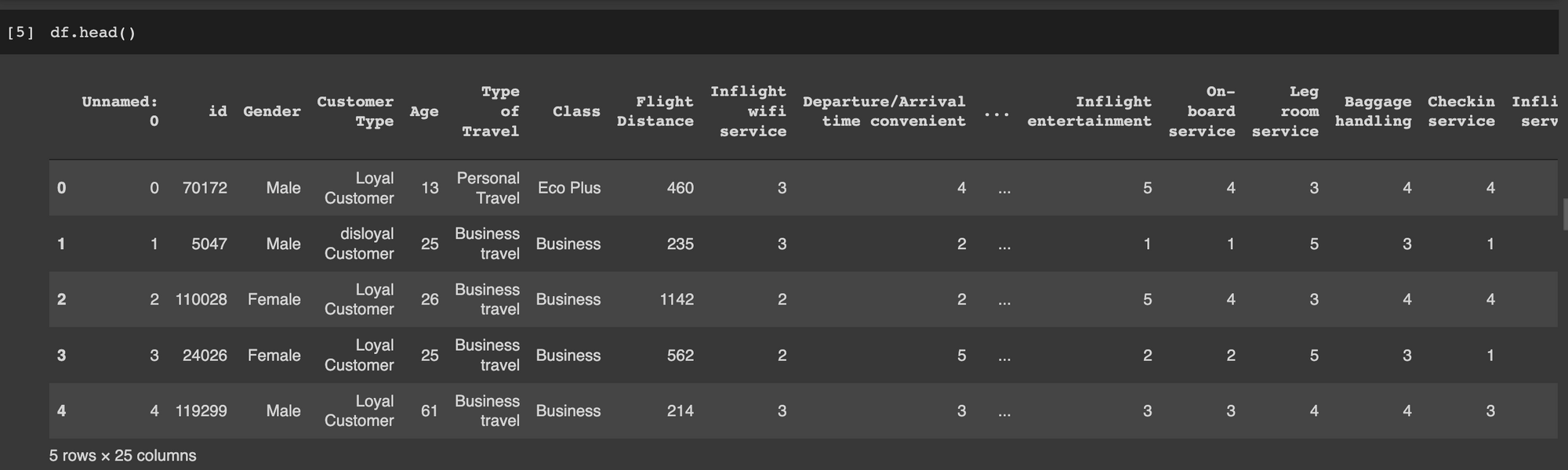
Data pre-processing
Ensure the data is clean before passing it to the neural network. For instance, we need to check for null values and deal with them. The occurrence of null values in the training data leads to nans in the training loss. The Arrival Delay in Minutes column has null values. There are various ways of dealing with null values, but in this case, we'll replace them with the mean of the column.
df['Arrival Delay in Minutes'] = df['Arrival Delay in Minutes'].mean()The target column is a string.
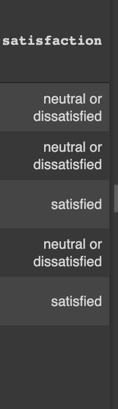
We can't pass strings to the neural network. Convert this column to a numerical representation. This can be done using Scikit-learn's label encoder.
from sklearn.preprocessing import LabelEncoder
labelencoder = LabelEncoder()
df = df.assign(satisfaction = labelencoder.fit_transform(df["satisfaction"]))
Data transformation
Apart from the target column, other columns are also in text form. They need to be converted to a numerical format.
categories = df.select_dtypes(include=['object']).columns.tolist()
categories
#['Gender', 'Customer Type', 'Type of Travel', 'Class']
Another thing we need to do is to scale the dataset. The weights and biases of neural networks are initialized to small numbers, usually between 0 and 1. Scaling makes training easier by forcing all values to be within a certain range. Failure to scale can lead to nans in the training loss due to the large magnitude between training values. After doing all this, we'll split the data into a training and testing set.
Let's use the ColumnTransformer from Scikit-learn to apply the transformations we have mentioned above. The transformer enables us to apply more than one transformation to multiple columns. In this case, we apply the following steps:
- Transform categorical columns to numerical form via one-hot encoding.
- Scale numerical columns using
MinMaxScalerto ensure that all values are between 0 and 1.
After obtaining the transformed data, we split it into a training and testing set.
from sklearn.model_selection import train_test_split
from sklearn.preprocessing import MinMaxScaler
X = df.drop(["Unnamed: 0", "id","satisfaction"], axis=1)
y = df["satisfaction"]
random_state = 13
test_size = 0.3
transformer = ColumnTransformer(transformers=[('cat', OneHotEncoder(handle_unknown='ignore', drop="first"), categories)],remainder=MinMaxScaler())
X = transformer.fit_transform(X)
X_train, X_test, y_train, y_test = train_test_split(X, y, test_size=test_size,random_state=random_state)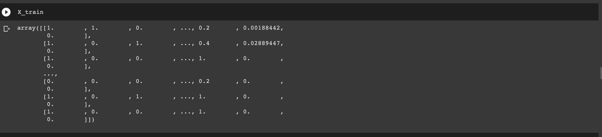
How to build the artificial neural network
Keras makes it easy to design neural networks via the Sequential API. We can stack the layers we want in our network using this API. In this case, let's define a network with the following layers:
- Input layer with the number of units similar to the number of features in the training data.
- Two dense layers. We randomly define the units in these layers, but we'll look at how to select the best units later.
- A final dense with 1 unit and the sigmoid activation function because it's a binary classification problem.
model = Sequential(
    [
        Input(shape=(X_train.shape[1],)),
        Dense(64, activation="relu",  kernel_initializer="glorot_uniform",name="layer1"),
        Dense(32, activation="relu", kernel_initializer="glorot_uniform", name="layer2"),
        Dense(1, activation="sigmoid", name="layer3"),
    ]
)
Apart from the number of units, the dense layer has other parameters:
- Activation function, usually ReLu.
- The kernel initializer that determines how the weights will be initialized.
namefor naming each layer.
The next step is to compile the neural network. This is where gradient descent is applied. This is the optimization strategy that reduces the errors as the network is learning. There are various optimization strategies but adam is a common approach. It applies the Adam algorithm.
model.compile(optimizer="adam", loss="binary_crossentropy", metrics=["accuracy"]) The next step is to train the network. Training is done using the fit method. It expects the following parameters:
- The training data.
- The validation data.
- The number of samples to be passed to the network at one time. This is declared using
batch_size. - The number of epochs to train the network.
history = model.fit(X_train, y_train, validation_data =(X_test, y_test), batch_size = 32, epochs = 100)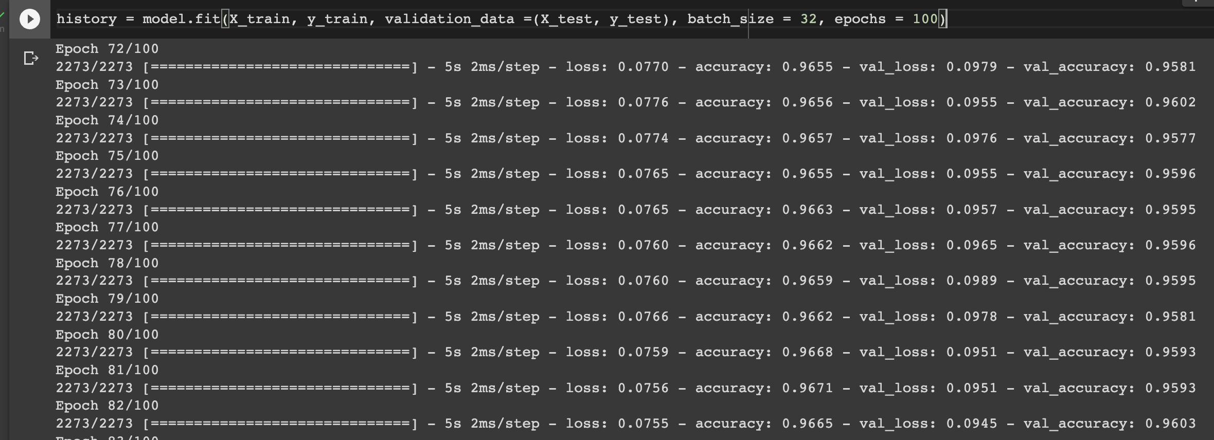
How to visualize model performance
Notice that we assigned the training function to the history variable. This variable now contains the training and validation metrics. We can use these variables to visualize the neural network's performance using Matplotlib.
metrics_df = pd.DataFrame(history.history)
metrics_df[["loss","val_loss"]].plot();
metrics_df[["accuracy","val_accuracy"]].plot();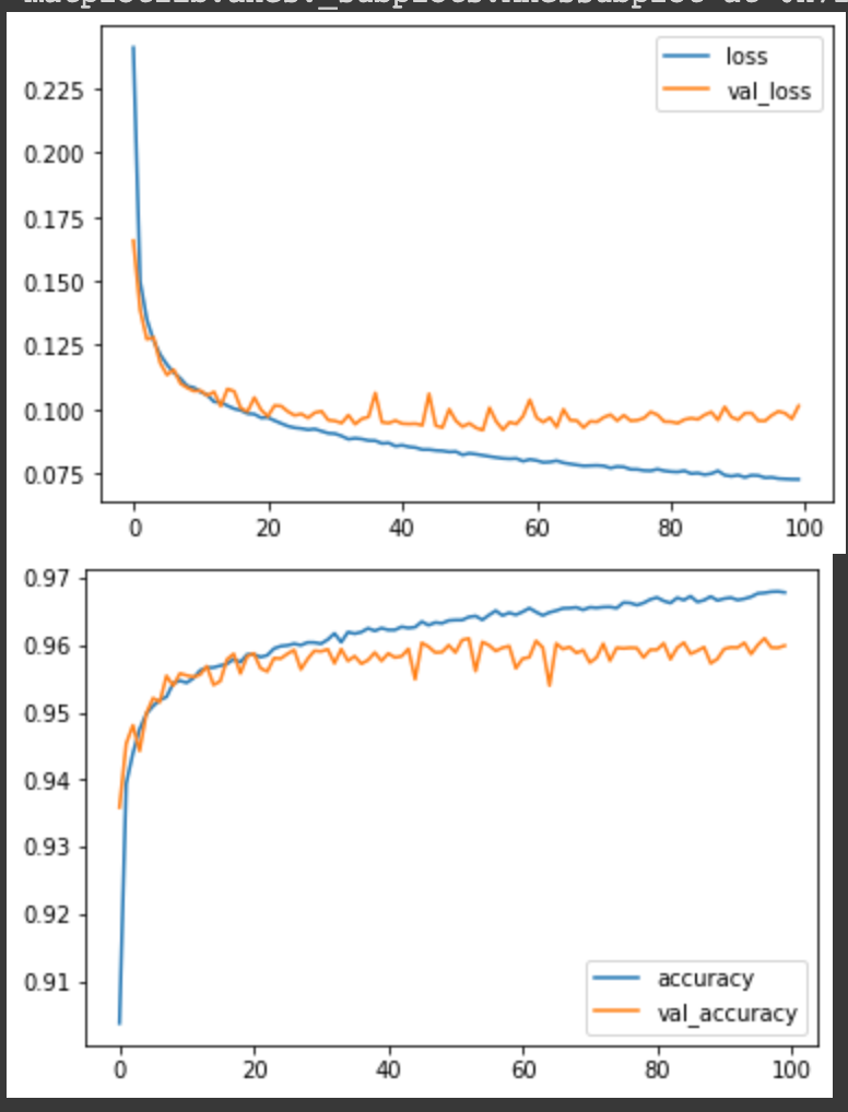
You can tell the network is learning if the training and validation loss decreases gradually. If the network is performing significantly worse on the test data compared to the training data, then it means that it's overfitting on the training data. Overfitting means that the network cannot determine patterns in the training data but memorizes it. As a result, it performs worse on data it hasn't seen during training. You can avoid overfitting by adding a dropout layer.
Read more: TensorBoard tutorial (Deep dive with examples and notebook)
Add dropout regularization to fight overfitting
A dropout layer ensures that some connections are "dropped" during the training process. This forces the network to learn the patterns in the data instead of memorizing the data. Therefore, the network performs well even on data it hasn't seen. In this case, we add a Dropout layer and specify that 1% of the connections should be dropped.
from tensorflow.keras.layers import Dropout
model = Sequential(
    [
        Input(shape=(X_train.shape[1],)),
        Dense(64, activation="relu",  kernel_initializer="glorot_uniform",name="layer1"),
        Dropout(rate=0.1),
        Dense(32, activation="relu", kernel_initializer="glorot_uniform", name="layer2"),
        Dense(1, activation="sigmoid", name="layer3"),
    ])
model.compile(optimizer="adam", loss="binary_crossentropy", metrics=["accuracy"])
history = model.fit(X_train, y_train, validation_data =(X_test, y_test), batch_size = 32, epochs = 10)
How to accelerate network training with batch normalization
As the name suggests, batch normalization — batchnorm – involves normalizing the input to the network. Batch normalization ensures that the mean output is close to o and the output standard deviation is close to 1. It normalizes input using the mean and standard deviation of the current training batch. When making predictions, batch normalization normalizes its output using the moving average of the mean and standard deviation of the batches computed during training. Batch normalization is primarily applied in deep neural networks to make training faster.
from tensorflow.keras.layers import BatchNormalization
model = Sequential(
    [
        Input(shape=(X_train.shape[1],)),
        Dense(64, activation="relu",  kernel_initializer="glorot_uniform",name="layer1"),
        BatchNormalization(),
        Dense(32, activation="relu", kernel_initializer="glorot_uniform", name="layer2"),
        Dense(1, activation="sigmoid", name="layer3"),
    ]
)
model.compile(optimizer="adam", loss="binary_crossentropy", metrics=["accuracy"])
history = model.fit(X_train, y_train, validation_data =(X_test, y_test), batch_size = 32, epochs = 10)
How to stop model training at the right time with early stopping
When training neural networks, it's often good practice to stop the training when the model's performance is no longer improving. In TensorFlow, this is achieved using the EarlyStopping callback. By default, the callback will monitor the loss and halt training when the loss is no longer improving for the number of epochs specified. In this case, we stop training if the loss is not decreasing for three consecutive epochs.
model.compile(optimizer="adam", loss="binary_crossentropy", metrics=["accuracy"])
callbacks = [tf.keras.callbacks.EarlyStopping(monitor='loss', patience=3)]
history = model.fit(X_train, y_train, validation_data =(X_test, y_test), batch_size = 32, epochs = 100,callbacks=callbacks)
How to save the best model with checkpoints
Apart from halting the training, you may want to save the best model as the network is training. You can do this with a checkpoint callback. The checkpoint callback expects:
- The path where the model will be saved.
- The metric to monitor.
save_best_onlyto dictate how the model will be saved. If true, the best model is saved.save_weights_onlyto determine if the entire model will be saved or just the weights. In this case, we save the weights only.modeis set tomaxhere because we are monitoring the validation accuracy.
checkpoint_filepath = "model_checkpoint"
model.compile(optimizer="adam", loss="binary_crossentropy", metrics=["accuracy"])
callbacks = [

             tf.keras.callbacks.EarlyStopping(monitor="loss", patience=3),

             tf.keras.callbacks.ModelCheckpoint(
             filepath=checkpoint_filepath,
             save_weights_only=True,
             monitor="val_accuracy",
             mode="max",
             save_best_only=True)]

history = model.fit(X_train, y_train, validation_data =(X_test, y_test), batch_size = 32, epochs = 10,callbacks=callbacks)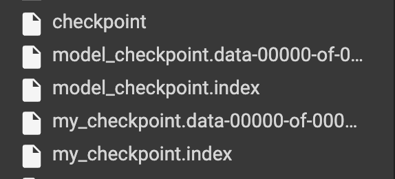
When training is complete, we can load the model with the weights saved by the checkpoint.
model.load_weights(checkpoint_filepath)Make predictions on the test set
Let's now use this model to make predictions on the test set. We set the threshold for a positive prediction at 50%.
y_pred = model.predict(X_test)
y_pred = (y_pred > 0.5)
Check the confusion matrix
We can use the above predictions to compute the confusion matrix.
from sklearn.metrics import confusion_matrix
cm = confusion_matrix(y_test, y_pred)
cm
# array([[17396,   387],
#       [  856, 12533]])
Make a single prediction
Let's demonstrate how to make a single prediction by selecting a sample from the test set. We use NumPy to expand the dimensions to include the batch size; in this case, it's 1.
import numpy as np
test_data = np.expand_dims(X_test[0], axis=0)
model.predict(test_data) > 0.5
# array([[ True]])
How to save and load Keras models
Apart from saving models using a checkpoint callback, you can also save them once training is complete. This is done using the save_weights function. The function expects the path where the model should be saved. This path should not be checkpoint as it will conflict with TensorFlow's default setting. Using checkpoint results in the error below.
model.save_weights('checkpoint')
# RuntimeError: Save path 'checkpoint' conflicts with path used for
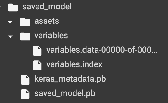
# checkpoint state. Please use a different save path.The save_weights functions will only save the model weights. To save the entire model, use model.save and pass the folder where the model should be stored. This saves the model weights, architecture, and training configuration. The optimizer and the training state are also saved, making it possible to restart training at the point where it stopped. By default, the model will be saved using the SavedModel format, but you can also use the HDF5 format.
model.save_weights('./checkpoints/my_checkpoint')
model.save("saved_model")
The directory where the entire model is saved contains the following items:
saved_model.pbthat store the training configuration and model architecture. The training configuration includes metrics, losses, and losses.-
variablesthat store the model weights.
You can then load the model and check its architecture.
new_model = tf.keras.models.load_model('saved_model')
new_model.summary()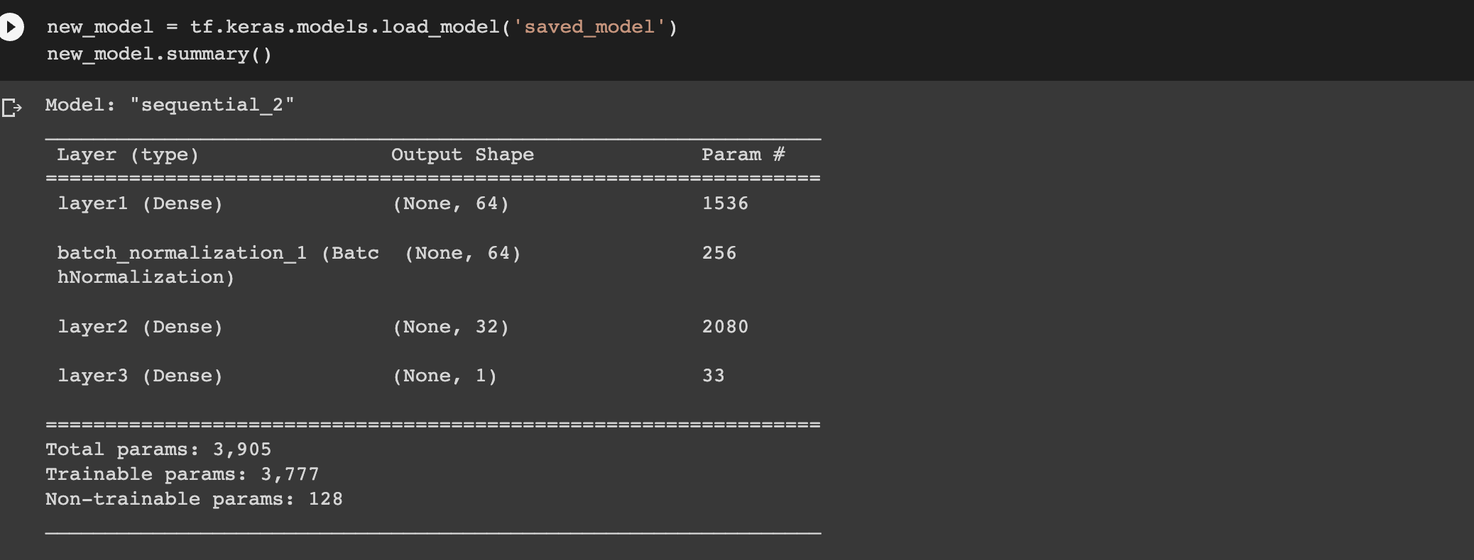
You can also save the model in HDF5 format.
# pip install pyyaml h5py  # Required to save models in HDF5 format
model.save('my_model.h5')
new_model = tf.keras.models.load_model('my_model.h5')
How to evaluate the Keras model with cross-validation
Next, let's look at how we can evaluate the Keras model with cross-validation. To achieve this, we apply the cross_val_score from Scikit-learn. The function expects:
- The training data.
- The scoring method.
- The cross-validation strategy to be used. A 5-fold cross-validation is used by default. The Stratified KFold strategy is applied if you specify an integer.
The SciKeras library enables the wrapping of Keras models as Scikit-learn models, making it possible to operate on the networks as if they were Scikit-learn models.
Install the package and import the KerasClassifier wrapper.
# pip install scikeras[tensorflow]
# https://www.adriangb.com/scikeras/stable/
from scikeras.wrappers import KerasClassifier
from sklearn.model_selection import cross_val_score
KerasClassifier expects a Keras model. We, therefore, create a function that returns a Keras model.
def make_model():
  model = Sequential([
        Input(shape=(X_train.shape[1],)),
        Dense(64, activation="relu",  kernel_initializer="glorot_uniform",name="layer1"),
        Dense(32, activation="relu", kernel_initializer="glorot_uniform", name="layer2"),
        Dense(1, activation="sigmoid", name="layer3"), ])
  return model
Next, we instantiate the classifier using this function.
model = KerasClassifier(model=make_model, batch_size=32, optimizer="adam", metrics=["accuracy"],loss="binary_crossentropy",validation_split=0.2, epochs=1)Apart from the model function, the classifier expects:
- The metrics.
- The loss.
- The validation split.
- The optimizer.
- The number of epochs.
By default, the KerasClassifier will compile the model. You can, however, compile the model in the make_model function.
Let's now apply cross_val_score and obtain the mean of the accuracy and standard deviation.
accuracies = cross_val_score(estimator=model, X=X_train, y=y_train, cv = 10, n_jobs = -1)
mean = accuracies.mean()
mean
# 0.9180552089621082
variance = accuracies.var()
variance
# 8.615227293449488e-05
How to tune model hyperparameters in Keras
One common strategy for hyperparameter tuning is grid search which performs an exhaustive search on the given parameters. Random search is an alternative that performs a randomized search on the given parameters. In this case, let's apply grid search.
The first step is to define the parameters to search over.
params = {
    "batch_size":[10,20,32,64],
    "epochs":[2,3,4],
    "optimizer":["adam","rmsprop"]
}
Next, create an instance of GridSearchCV. It expects:
- The estimator.
- The parameters.
- The scoring criteria.
- The cross-validation method to be applied. By default, it applies K-Fold cross-validation. When an integer is passed, it applies the Stratified K-Fold cross-validation.
grid_search = GridSearchCV(estimator=model,
                           param_grid=params,
                           scoring="accuracy",
                           cv=2)
The next step is to fit the grid search to the training data.
grid_search = grid_search.fit(X_train,y_train)When it's complete, we can check the best parameters.
best_param = grid_search.best_params_
best_param
# {'batch_size': 20, 'epochs': 4, 'optimizer': 'adam'}
best_accuracy = grid_search.best_score_
best_accuracy
# 0.9392839465434747
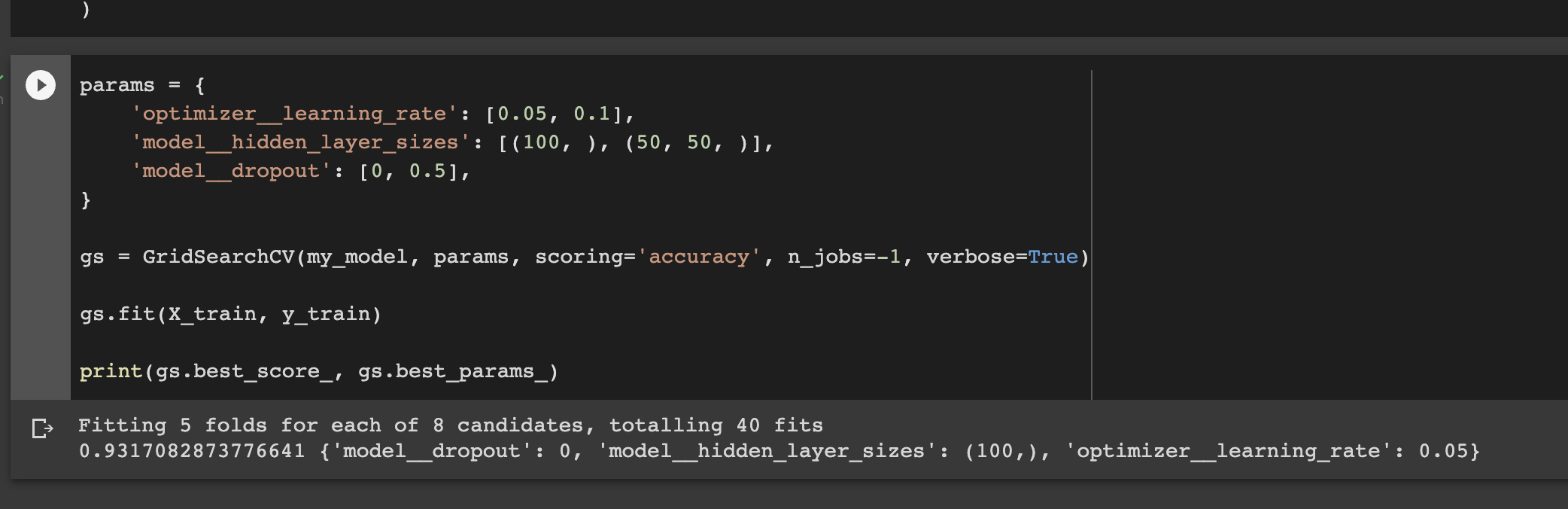
How to tune the network parameters
It is also possible to tune the parameters of the network, for example, the number of hidden layers and the dropout rate. The first step is to define the model function with hidden_layer_sizes and dropout as parameters.
def make_clf(hidden_layer_sizes, dropout):
    model = Sequential()
    model.add(Input(shape=(X_train.shape[1],)))
    for hidden_layer_size in hidden_layer_sizes:
        model.add(Dense(hidden_layer_size, activation="relu"))
        model.add(Dropout(dropout))
    model.add(Dense(1, activation="sigmoid"))
    return model
The next step is to define the parameters to be tested and perform the search as you have done before. Thereafter, print the best_score_ and the best_params. By default, the refit parameter of GridSearchCV is True meaning that the model will be re-trained with the best parameters. Therefore, once GridSearchCV is over, the model is ready for making predictions.
params = {
    'optimizer__learning_rate': [0.05, 0.1],
    'model__hidden_layer_sizes': [(100, ), (50, 50, )],
    'model__dropout': [0, 0.5],
}

gs = GridSearchCV(my_model, params, scoring='accuracy', n_jobs=-1, verbose=True)

gs.fit(X_train, y_train)

print(gs.best_score_, gs.best_params_)
# 0.9317082873776641 {'model__dropout': 0, 'model__hidden_layer_sizes': (100,), 'optimizer__learning_rate': 0.05}
Final thoughts
This article has been an in-depth guide to deep learning and building neural networks with TensorFlow and Keras. We have covered some core concepts to get you started with deep learning in TensorFlow. You have also learned:
- Which activation function to apply in a deep learning network.
- Which activation function to apply in the hidden and output layers.
- Selecting the appropriate loss function.
- How neural networks learn through gradient descent and backpropagation.
- TensorFlow basics.
- How TensorFlow works.
- Training a neural network with Keras and TensorFlow.
- Performing hyperparameter tuning and cross-validation on the neural network, among other topics.
TensorFlow resources
Object detection with TensorFlow 2 Object detection API
How to create custom training loops in Keras
How to train deep learning models on Apple Silicon GPU
How to build CNN in TensorFlow(examples, code, and notebooks)
The Complete Data Science and Machine Learning Bootcamp is a great next step if you want to keep exploring the data science and machine learning field.
Follow us on LinkedIn, Twitter, GitHub, and subscribe to our blog, so you don't miss a new issue.