
TensorBoard tutorial (Deep dive with examples and notebook)


TensorBoard is a visualization library that enables data science practitioners to visualize various aspects of their machine learning modeling. For instance, you can use TensorBoard to:
- Visualize the performance of the model.
- Tuning model parameters.
- Profile the executions of the program. For example, check the utilization of GPUs.
- Debug machine learning code.
TensorBoard can be used with various machine learning libraries such as TensorFlow, PyTorch, Flax, and XGBoost. Let's dive in and see how to use TensorBoard with all these packages.
mlnuggets newsletter
Join the newsletter to receive the technical deep dives in your inbox.
Advantages of using Tensorboard
The main advantages of using Tensorboard include:
- Allows data scientists to visualize the construction of neural networks, thus driving better problem-solving.
- Enables tracking of the performance of machine learning models using metrics such as accuracy and log loss on training or validation sets.
- Easy debugging of the neural nodes.
How to use TensorBoard
Let's look at how you can start using TensorBoard.
How to install TensorBoard
To get started, install TensorBoard, which can be done using pip or conda.
PIP installation
Run the following command on the terminal or command prompt:
pip install tensorboardAlternatively, in Jupyter Notebook:
!pip install tensorboardConda installation
Open the Anaconda command prompt and run any of the following commands:
conda install tensorboard
Docker installation
If you use a Docker image of the Jupyter Notebook server, expose the notebook's and TensorBoard's ports. To do so, run the following command:
docker run -it -p 8888:8888 -p 6006:6006 \ tensorflow/tensorflow:nightly-py3-jupyter mlnuggets newsletter
Join the newsletter to receive the technical deep dives in your inbox.
Using TensorBoard with Jupyter notebooks and Google Colab
To install Jupyter Notebook, either install it using Anaconda or through pip:
pip install notebookAfter installing the Jupyter Notebook, start an instance of a notebook:
jupyter notebookIf you prefer using Google Colab, go to https://colab.research.google.com/ and create a new notebook instance.
You are now set to use TensorBoard. Run the following command in a notebook instance (Jupyter or Google Colab):
%load_ext tensorboard To reload a TensorBoard that had been previously loaded, run:
%reload_ext tensorboardNext, set the log directory where all the logs will be stored. Logs refer to the data that will be used to generate visualizations. If you are using Jupyter Notebook in a Linux distribution, remove the existing logs:
rm -rf ./logs/ If you are using Google Colab.
!rm -rf ./logs/For users running TensorBoard from a Jupyter Notebook on a Windows machine, run the following code:
#rm -rf ./logs/

#for windows
import shutil
try:
    shutil.rmtree('logs')
except:
    pass

#for windows
import shutil
try:
    shutil.rmtree('logsx')
except:
    pass
Now create a directory where you can store the logs.
log_dir = "logs/model_fit/" + datetime.datetime.now().strftime("%Y%m%d-%H%M%S")Adding a datetime enables the storage and comparison of logs at different run times.
mlnuggets newsletter
Join the newsletter to receive the technical deep dives in your inbox.
How to run TensorBoard
To demonstrate model visualization in Tensorboard, including metrics, consider the iris data classification problem, which involves classifying iris plants into three classes.
First, load the TensorBoard extension:
%load_ext tensorboard Then define the model:
import datetime
from sklearn.preprocessing import normalize
import numpy as np
from sklearn import datasets
import tensorflow as tf
#LOaD DATA
iris = datasets.load_iris()
X = iris.data
y = iris.target
#normalize
X  =  normalize(X,axis = 0)


#Neural network module
from keras.models import Sequential
import keras
from keras.layers import Dense,Activation,Dropout
import tensorflow
from tensorflow.keras.layers import BatchNormalization
from keras.utils import np_utils
import os


from sklearn.model_selection import train_test_split
# Load the iris dataset
iris = datasets.load_iris()
X = iris.data
y = iris.target
# Create training and test split

'''
70% -- train y
30% -- test y
'''

X_train, X_test, y_train, y_test = train_test_split(X, y, test_size=0.3, stratify=y, random_state=42)
X_train1, X_test1, y_train1, y_test1 = X_train, X_test, y_train, y_test
# Create categorical labels
y_train = np_utils.to_categorical(y_train)
y_test = np_utils.to_categorical(y_test)


def create_model():
    # Create the model
    model = keras.models.Sequential()
    model.add(Dense(512, activation='relu', input_shape=(4,)))
    model.add(Dense(3, activation='softmax'))
    # Compile the model
    model.compile(optimizer='rmsprop',
                    loss='categorical_crossentropy',
                    metrics=['accuracy'])
    return model
create_model()
Create and compile the model.
logdir = os.path.join("logs", datetime.datetime.now().strftime("%Y%m%d-%H%M%S"))

tensorboard_callback = tf.keras.callbacks.TensorBoard(logdir, histogram_freq=1)

def train_model():
    '''
    utility function for training the model
    '''

    model = create_model()

    tensorboard_callback = tf.keras.callbacks.TensorBoard(logdir, histogram_freq=1)
    model.fit(x=X_train,
            y=y_train,
            epochs=10,
            validation_data=(X_test, y_test), callbacks = tensorboard_callback)
    #
    # Get the accuracy of test data set
    #
    test_loss, test_acc = model.evaluate(X_test, y_test)
    #
    # Print the test accuracy
    #
    print('Test Accuracy: ', test_acc, '\nTest Loss: ', test_loss)

tf.debugging.experimental.enable_dump_debug_info(
    "/tmp/tfdbg2_logdir",
    tensor_debug_mode="FULL_HEALTH",
    circular_buffer_size=-1)
#train the model
train_model()
Now load the TensorBoard notebook extension and define a variable log_folder that points to the logs folder that you had created.
%load_ext tensorboard log_folder = 'logs'How to use TensorBoard callback
A callback is an object that carries out operations over various stages of training, such as:
- At the end of an epoch.
- Before or after a specified number of batches.
on_batch_begin– when a batch begins.on_batch_end– when a batch ends.on_train_begin– when training begins.on_train_end– when training ends.
TensorBoard callback creates a log for the TensorBoard, including:
- Plots summarizing metrics.
- Training graph visualization.
- Weight histograms.
- Sampled profiling.
When used in Model.evaluate, additional components apart from epochs, there will be summaries that show the distribution of evaluation metrics vs Model.optimizer.iterations. Metrics are prepended with the corresponding evaluation, with model.optimizer.iterations being the step in the visualized TensorBoard.
Import TensorBoard.
from tensorflow.keras.callbacks import TensorBoard Create the TensorBoard callback.
logdir = os.path.join("logs", datetime.datetime.now().strftime("%Y%m%d-%H%M%S"))

tensorboard_callback = tf.keras.callbacks.TensorBoard(logdir, histogram_freq =  1, write_graph = False,write_images = False)
You can include other parameters such as:
write_graph– specifies whether to visualize a graph in TensorBoard. It results in a larger log file if set toTrue.write_images– specifies whether to write model weights to visualize as an image in TensorBoard.write_steps_per_second– specifies whether to log training steps per second into TensorBoard. Can be used with either epoch or batch frequency logging.update_freq–batchorepochorinteger. When usingbatch, losses and metrics are written to TensorBoard after each batch. Similar to whenepochis specified. If you specifyinteger, for example, 1000, the metrics and losses are saved to TensorBoard every 1000 batches.profile_batch– a non-negative integer or tuple of integers that profiles a batch(es) to sample compute characteristics. Profiling is disabled by default.embeddings_freq– frequency (in epochs) at which embedding layers are visualized. If set to 0, there is no visualization of the embeddings.embeddings_metadata– a dictionary that maps embedding layer names to the filename where the metadata for the embedding layer is saved. A single filename can be passed if the same metadata file is used for all embedding layers.histogram_freq– the frequency at which to compute activation and weight histograms for layers of the trained model.
The next step involves compiling and fitting the model using the callbacks, which will store information in the logs.
from tensorflow import keras
logdir = "logs/scalars/" + datetime.datetime.now().strftime("%Y%m%d-%H%M%S")
file_writer = tf.summary.create_file_writer(logdir + "/metrics")
file_writer.set_as_default()


tensorboard_callback = keras.callbacks.TensorBoard(log_dir=logdir, histogram_freq=1)

def train_model():
    '''
    utility function for training the model
    '''

    model = create_model()

    tensorboard_callback = tf.keras.callbacks.TensorBoard(logdir, histogram_freq=1)
    model.fit(x=X_train,
            y=y_train,
            epochs=20,
            validation_data=(X_test, y_test), callbacks = [tensorboard_callback])
    #
    # Get the accuracy of test data set
    #
    test_loss, test_acc = model.evaluate(X_test, y_test)
    #
    # Print the test accuracy
    #
    print('Test Accuracy: ', test_acc, '\nTest Loss: ', test_loss)
train_model()
Once the model is trained, the next step is to visualize it using TensorBoard. For that, data from the logs stored through callbacks will be used.
mlnuggets newsletter
Join the newsletter to receive the technical deep dives in your inbox.
How to launch TensorBoard
You can launch the TensorBoard extension via the command prompt.
tensorboard --logdir logs Alternatively, you can launch TensorBoard in Jupyter Notebook or Google Colab:
%tensorboard --logdir logs The TensorBoard can also be accessed through the local host http://localhost:6006 or http://127.0.0.1:6006/
If you have set everything right, you will see a window with interactive functionality like the one shown below.
Running TensorBoard remotely
It is common practice to experiment remotely on a server with GPUs, especially when the Tensorflow model requires a lot of computational resources. To use TensorBoard on a remote server:
- Initiate an SSH to access the TensorBoard web user interface. On the command prompt, run:
ssh -L 6006:127.0.0.1:6006 username@server_ipIf you are using PuTTY, you will need to replace ssh in the command with PuTTY to create an ssh tunnel on port 6006 from the local machine to port 6006 on the server that you connected to with SSH. The tunnel you have created will stay open while the SSH connection is active.
2. Next, from the browser, you can access TensorBoard through http://localhost:6006 or http://127.0.0.1:6006/
However, sometimes you need to contact the server and then use the contact to connect to the server GPU. In such a case, you will add an extra step to the transfer port:
- Transfer port from contact server to the local machine using SSH. In your local machine:
ssh -L 6006:127.0.0.1:6006 username@contact_server_ip2. Transfer the port from the GPU server to the contact. Your server:
ssh -L 6006:127.0.0.1:6006 username@GPU_server_ip3. Now start the TensorBoard on the GPU server.
tensorboard --logdir = './tensorboard_dirs' --port = 6006mlnuggets newsletter
Join the newsletter to receive the technical deep dives in your inbox.
TensorBoard dashboards
As shown in the Sample dashboard earlier, various components are included in a single dashboard. These components include:
- TensorBoard scalars.
- Images.
- Graphs.
- Distributions.
- Histograms.
- Fairness indicators.
- What-If Tool (WIT).
Each of these components provides information regarding the model, as illustrated below.
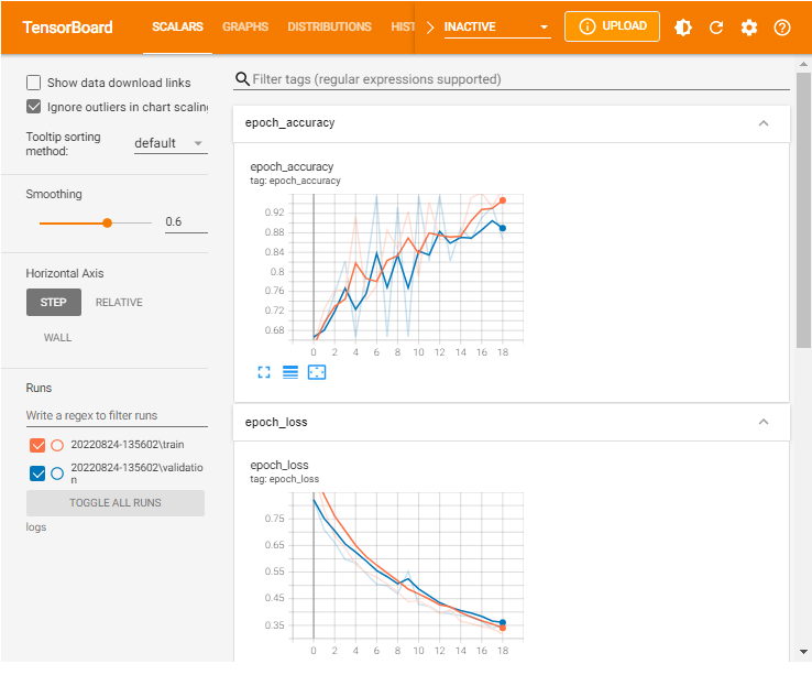
TensorBoard scalars
The TensorBoard scalars dashboard visualizes scalar statistics such as classification accuracy, model loss, or learning rate.
from tensorflow import keras
logdir = "logs/scalars/" + datetime.datetime.now().strftime("%Y%m%d-%H%M%S")
file_writer = tf.summary.create_file_writer(logdir + "/metrics")
file_writer.set_as_default()


tensorboard_callback = keras.callbacks.TensorBoard(log_dir=logdir, histogram_freq=1)

def train_model():
    '''
    utility function for training the model
    '''

    model = create_model()

    tensorboard_callback = tf.keras.callbacks.TensorBoard(logdir, histogram_freq=1)
    model.fit(x=X_train,
            y=y_train,
            epochs=20,
            validation_data=(X_test, y_test), callbacks = [tensorboard_callback])
    #
    # Get the accuracy of test data set
    #
    test_loss, test_acc = model.evaluate(X_test, y_test)
    #
    # Print the test accuracy
    #
    print('Test Accuracy: ', test_acc, '\nTest Loss: ', test_loss)
train_model()Load TensorBoard.
%tensorboard --logdir logs/scalars
You can also include custom scalars. For instance, if you want to have a custom learning rate that decreases as epochs increase, you can define a function as shown below.
def lr_schedule(epoch):
    """
    Returns a custom learning rate that decreases as epochs progress.
    """
    learning_rate = 0.2
    if epoch > 10:
        learning_rate = 0.02
    if epoch > 20:
        learning_rate = 0.01
    if epoch > 50:
        learning_rate = 0.005

    tf.summary.scalar('learning rate', data=learning_rate, step=epoch)
    return learning_rate

lr_callback = keras.callbacks.LearningRateScheduler(lr_schedule)

tensorboard_callback = keras.callbacks.TensorBoard(log_dir=logdir)

def train_model(epochs = 20):
    '''
    utility function for training the model
    '''

    model = create_model()

    tensorboard_callback = tf.keras.callbacks.TensorBoard(logdir, histogram_freq=1)
    model.fit(x=X_train,
            y=y_train,
            epochs=epochs,
            validation_data=(X_test, y_test), callbacks = [tensorboard_callback, lr_callback])
    #
    # Get the accuracy of test data set
    #
    test_loss, test_acc = model.evaluate(X_test, y_test)
    #
    # Print the test accuracy
    #
    print('Test Accuracy: ', test_acc, '\nTest Loss: ', test_loss)

train_model(4) Next, load TensorBoard.
%tensorboard --logdir logs/scalarsNotice that now you have a new scalar output– learning rate
mlnuggets newsletter
Join the newsletter to receive the technical deep dives in your inbox.
TensorBoard images
Tensorboard allows you to display images using tf.summary and tf.summary.image. Consider the case of the popular MNIST dataset. You can display the image as shown below.
#import libraries
import itertools
import datetime
import io
import tensorflow as tf
from tensorflow import keras
import matplotlib.pyplot as plt
import numpy as np
import sklearn.metrics
import shutil

try:
    shutil.rmtree('logsx')
except:
    pass

fashion_mnist = keras.datasets.fashion_mnist
(train_images, train_labels), (test_images, test_labels) = fashion_mnist.load_data()

# Names of the integer classes
class_names = ['T-shirt/top', 'Trouser', 'Pullover', 'Dress', 'Coat',
    'Sandal', 'Shirt', 'Sneaker', 'Bag', 'Ankle boot']

# Reshape the image for the Summary API.
img = np.reshape(train_images[100], (-1, 28, 28, 1))

# Sets up a timestamped log/images directory.
logdir = "logsx/images/" + datetime.datetime.now().strftime("%Y%m%d-%H%M%S")
# Creates a file writer for the log directory.
file_writer = tf.summary.create_file_writer(logdir)

# Using the file writer, log the reshaped image
with file_writer.as_default():
    tf.summary.image("Image data", img, step=0)
%reload_ext tensorboard
%tensorboard --logdir logsx/images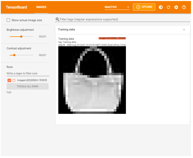
You can also display multiple images using the max_outputs. The max_outputsargument specifies the number of images you want to visualize.
with file_writer.as_default():
    # Don't forget to reshape.
    images = np.reshape(train_images[50:53], (-1, 28, 28, 1))
    tf.summary.image("Plotting multiple images", images, max_outputs=3, step=0)

%tensorboard --logdir logsx/images
TensorBoard graphs
The graphing component of TensorBoard can be helpful in model debugging. To see the graph from TensorBoard, click on the GRAPHS tab in the upper pane. From the upper left corner, select your preferred run. You can view the model and align it with your desired design.
You will notice options like an op-level graph that gives you insight into how to change your model. Turning on the trace inputs node option shows the upstream dependencies of that node.
mlnuggets newsletter
Join the newsletter to receive the technical deep dives in your inbox.
TensorBoard distributions
Deep neural network models(DNN) are made up of many layers. Each layer of a DNN comprises biases and weights. Distributions display the distribution of the biases and weights.
TensorBoard histograms
TensorBoard histograms are a collection of values aggregated by frequency. TensorBoard histograms visualize weights over time. Hence, they help establish whether there is something wrong with weights initialization or the learning rate. Histograms are located in the HISTOGRAM tab.
You can specify the histogram mode as either OVERLAY:
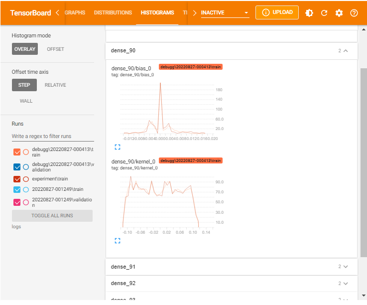
or OFFSET histogram:
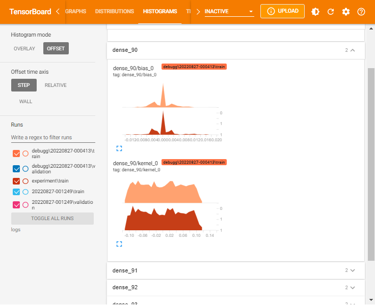
As shown, Histograms display similar information as the Distributions but as a 3-D histogram changing across various iterations.
mlnuggets newsletter
Join the newsletter to receive the technical deep dives in your inbox.
Fairness indicators
Regardless of how much care has been taken during the model implementation and evaluation process, bias can happen at various stages in the model pipeline.
Therefore, it is essential to evaluate the model for human bias across all the steps. In Tensorboard, the Fairness Indicators enable developers to evaluate fairness metrics, such as False Positive Rate (FPR) and False Negative Rate (FNR), for binary and multi-class classification and regression models.
Install the Fairness Indicators plugin:
pip install --upgrade pip pip install fairness_indicators pip install tensorboard-plugin-fairness-indicators
You will need to restart the kernel for the plugin to be included in TensorBoard. The Fairness Indicators widget can be accessed from the dialog box:
 tensorflow
What-If Tool (WIT)
When building machine learning models, developers are often concerned with understanding when the model underperforms or performs well. The What-If Tool (WIT) comes in handy when you are interested in:
- Counterfactual reasoning.
- Investigating decision boundaries.
- Explore how general changes to data points affect predictions.
- Simulating various realities to determine how a model behaves from the tool's widget visual interface.
In Tensorboard, the What-If Tool can be configured from the dialog box. After opening the What If widget, you need to provide:
- The host and port of the model server.
- The name of the model being served.
- The type of model.
- The path to where you stored the TFRecords file to load.
Next, click Accept. The tool will do the rest and return the results.
Displaying data in TensorBoard
Various data formats are supported for logging and visualization in Tensorboard, including scalars, images, audio, histograms, and graphs.
Using the TensorBoard embedding projector
TensorBoard's projector facilitates easy interpretation and understanding of embeddings. By visualizing the high-dimensional embeddings, you understand the connection of embedding layers. This guide will consider a simple example of vectors and metadata. You will use the SummaryWriter to write the embedding by creating an instance and adding an embedding.
Delete previous logs.
!rm -rf runsCreate some vectors and metadata.
%load_ext tensorboard
import numpy as np
import tensorflow as tf
import tensorboard as tb
tf.io.gfile = tb.compat.tensorflow_stub.io.gfile
#install pytorch
#!pip install torch
from torch.utils.tensorboard import SummaryWriter


vectors = np.array([[0,0,1], [0,1,0], [1,0,0], [1,1,1], [1,0,1]])
metadata = ['001', '010', '100', '111', '101']  # labels
writer = SummaryWriter()
writer.add_embedding(vectors, metadata)

writer.close()

%tensorboard --logdir=runs
Load the TensorBoard dashboard and navigate to the Projector window.
%tensorboard --logdir logs/train_data
mlnuggets newsletter
Join the newsletter to receive the technical deep dives in your inbox.
Plot training examples with TensorBoard
Before fitting the training model, you can visualize training data as shown below.
from tensorflow import keras
#clear previous logs
!rm -rf logs/train_data
# Download the mnist data. The data is already divided into train and test.
# The labels are integers representing classes.
handwriting_mnist = keras.datasets.mnist
(train_images, train_labels), (test_images, test_labels) = \
    handwriting_mnist.load_data()

logdir = "logs/train_data/"

file_writer = tf.summary.create_file_writer(logdir)

import numpy as np

with file_writer.as_default():
    images = np.reshape(train_images[50:53], (-1, 28, 28, 1))
    tf.summary.image("3 Digits", images, max_outputs=3, step=0)
Load TensorBoard.
%tensorboard --logdir logs/train_data
Visualize images in TensorBoard
Instead of tensors, you might consider plotting arbitrary images in TensorBoard. To demonstrate this, consider the MNIST dataset.
# Clear out prior logging data.
!rm -rf logs/plots

logdir = "logs/plots/" + datetime.datetime.now().strftime("%Y%m%d-%H%M%S")
file_writer = tf.summary.create_file_writer(logdir)


# class names
class_names = ['0', '1', '2', '3', '4', '5', '6', '7', '8', '9']


def plot_to_image(figure):
    """Converts the matplotlib plot specified by 'figure' to a PNG image and
      returns it. The supplied figure is closed and inaccessible after this call."""
    # Save the plot to a PNG in memory.
    buf = io.BytesIO()
    plt.savefig(buf, format='png')
    # Closing the figure prevents it from being displayed directly inside
    # the notebook.
    plt.close(figure)
    buf.seek(0)
    # Convert PNG buffer to TF image
    image = tf.image.decode_png(buf.getvalue(), channels=4)
    # Add the batch dimension
    image = tf.expand_dims(image, 0)
    return image

def image_grid():
    """
      Return a 5x5 grid of the MNIST images as a matplotlib figure.
    """
    # Create a figure to contain the plot.
    figure = plt.figure(figsize=(10,10))
    for i in range(25):
        # Start next subplot.
        plt.subplot(5, 5, i + 1, title=class_names[train_labels[i]])
        plt.xticks([])
        plt.yticks([])
        plt.grid(False)
        plt.imshow(train_images[i], cmap=plt.cm.binary)

    return figure

# Prepare the plot
figure = image_grid()
# Convert to image and log
with file_writer.as_default():
    tf.summary.image("Image data", plot_to_image(figure), step=0)


%tensorboard --logdir logs/plots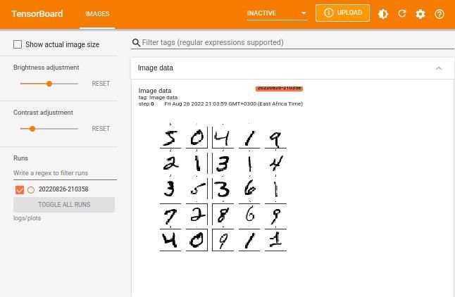
Displaying text data in TensorBoard
Using the TensorFlow Text Summary API, you can log textual data and visualize it in TensorBoard.
#define text to log
your_text = "This is some text in TensorBoard!"
# Remove prior log data.
!rm -rf logs

# Sets up a timestamped log directory.
logdir = "logs/text_basics/" + datetime.datetime.now().strftime("%Y%m%d-%H%M%S")
#log the writer to the logs directory.
file_writer = tf.summary.create_file_writer(logdir)

# Using the file writer, log the text.
with file_writer.as_default():
  tf.summary.text("TensorBoard Text", your_text, step=0)
Reload TensorBoard from the logs in the logs directory.
%tensorboard --logdir logs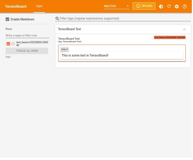
mlnuggets newsletter
Join the newsletter to receive the technical deep dives in your inbox.
Log confusion matrix to TensorBoard
You can log a confusion matrix and display the results as images. Sticking to the MNIST fashion dataset, log the confusion matrix as follows.
Clear previous logs
!rm -rf logsDownload and prepare the data.
#Importing Dataset
# downloading the dataset
fashion_mnist = keras.datasets.fashion_mnist
(train_images, train_labels), (test_images, test_labels) = fashion_mnist.load_data()

# all the classes
class_names = ('T-shirt/top', 'Trouser', 'Pullover', 'Dress', 'Coat',
        'Sandal', 'Shirt', 'Sneaker', 'Bag', 'Ankle Boot')

#train model
model = keras.models.Sequential([
   keras.layers.Flatten(input_shape=(28, 28)),
   keras.layers.Dense(512, activation='relu'),
   keras.layers.Dense(256, activation='relu'),
   keras.layers.Dense(128, activation='relu'),
   keras.layers.Dense(64, activation='relu'),
   keras.layers.Dense(32, activation='relu'),
   keras.layers.Dense(10, activation='softmax')
])
model.compile(loss='sparse_categorical_crossentropy', optimizer='adam', metrics=['accuracy'])
Create the function to log the confusion matrix using the LambdaCallback.
from tensorflow import keras
# Clearing out prior logging data.
!rm -rf logs/image
def plot_confusion_matrix(cm, class_names):
    figure = plt.figure(figsize=(8, 8))
    plt.imshow(cm, interpolation='nearest', cmap=plt.cm.Blues)
    plt.title("Confusion Matrix of the Results")
    plt.colorbar()
    tick_marks = np.arange(len(class_names))
    plt.xticks(tick_marks, class_names, rotation=90)
    plt.yticks(tick_marks, class_names)

    labels = np.around(cm.astype('float') / cm.sum(axis=1)[:, np.newaxis], decimals=2)

    threshold = cm.max() / 2.
    for i, j in itertools.product(range(cm.shape[0]), range(cm.shape[1])):
        color = "white" if cm[i, j] > threshold else "black"
        plt.text(j, i, labels[i, j], horizontalalignment="center", color=color)

    plt.tight_layout()
    plt.ylabel('Real Class')
    plt.xlabel('Predicted Class')
    return figure

logdir = "logs/image/" + datetime.datetime.now().strftime("%Y%m%d-%H%M%S")
# Defining the basic TensorBoard callback.
tensorboard_callback = keras.callbacks.TensorBoard(log_dir=logdir)
file_writer_cm = tf.summary.create_file_writer(logdir + '/cm')


def log_confusion_matrix(epoch, logs):
    # Using the model to predict the values from the validation dataset.
    test_pred_raw = model.predict(test_images)
    test_pred = np.argmax(test_pred_raw, axis=1)

    # Calculating the confusion matrix.
    cm = sklearn.metrics.confusion_matrix(test_labels, test_pred)
    figure = plot_confusion_matrix(cm, class_names=class_names)
    cm_image = plot_to_image(figure)

    with file_writer_cm.as_default():
        tf.summary.image("Confusion Matrix", cm_image, step=epoch)

# Defining the per-epoch callback.
cm_callback = keras.callbacks.LambdaCallback(on_epoch_end=log_confusion_matrix)
Train the model with the TensorFlow callback.
# Training the classifier.
model.fit(
   train_images,
   train_labels,
   epochs=2,
   verbose=0,
   callbacks=[tensorboard_callback, cm_callback],
   validation_data=(test_images, test_labels),
)
Load TensorBoard with the confusion matrix logs.
# Starting TensorBoard.
%tensorboard --logdir logs/image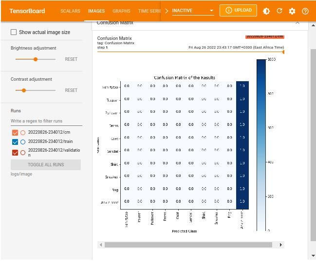
mlnuggets newsletter
Join the newsletter to receive the technical deep dives in your inbox.
Hyperparameter tuning with TensorBoard
Models are built with hyperparameters that influence the functionality of the model. You select the hyperparameters for optimization during modeling before settling for the 'best' model.
Some of these hyperparameters include number of epochs, dropout rate, or learning rate. Optimizing the selected hyperparameter is known as hyperparameter optimization or tuning. The goal is to improve the performance of the model.
To conduct hyperparameter tuning in TensorBoard, use the hparams plugin from Tensorboard. Consider the iris data classification problem.
Clear earlier logs.
#for kali
#rm -rf ./logs/

#for windows
import shutil
try:
    shutil.rmtree('logs')
except:
    pass

#for windows
import shutil
try:
    shutil.rmtree('logsx')
except:
    pass
Reload TensorBoard.
%reload_ext tensorboardDefine the hyperparameters you want to optimize and the data to train the model.
## Create hyperparameters
HP_NUM_UNITS=hp.HParam('num_units', hp.Discrete([ 5, 10]))
HP_DROPOUT=hp.HParam('dropout', hp.RealInterval(0.1, 0.2))
HP_LEARNING_RATE= hp.HParam('learning_rate', hp.Discrete([0.001, 0.0005, 0.0001]))
HP_OPTIMIZER=hp.HParam('optimizer', hp.Discrete(['adam', 'sgd', 'rmsprop']))
METRIC_ACCURACY='accuracy'
Set configuration files and store them in the logs directory.
'''Set configuration log files'''
log_dir ='logs/fit/' + datetime.datetime.now().strftime('%Y%m%d-%H%M%S')
with tf.summary.create_file_writer(log_dir).as_default():
    hp.hparams_config(
    hparams=
    [HP_NUM_UNITS, HP_DROPOUT,  HP_OPTIMIZER, HP_LEARNING_RATE],
    metrics=[hp.Metric(METRIC_ACCURACY, display_name='Accuracy')],
) Fit the models and include the log for metrics and hyperparameters.
def create_model(hparams):
    # Create the model
    model = keras.models.Sequential()
    model.add(Dense(512, activation='relu', input_shape=(4,)))
    model.add(Dense(3, activation='softmax'))

    #setting the optimizer and learning rate
    optimizer = hparams[HP_OPTIMIZER]
    learning_rate = hparams[HP_LEARNING_RATE]
    if optimizer == "adam":
        optimizer = tf.optimizers.Adam(learning_rate=learning_rate)
    elif optimizer == "sgd":
        optimizer = tf.optimizers.SGD(learning_rate=learning_rate)
    elif optimizer=='rmsprop':
        optimizer = tf.optimizers.RMSprop(learning_rate=learning_rate)
    else:
        raise ValueError("unexpected optimizer name: %r" % (optimizer_name,))

    # Comiple the mode with the optimizer and learninf rate specified in hparams
    model.compile(optimizer=optimizer,
              loss='categorical_crossentropy',
              metrics=['accuracy'])

    #Fit the model
    model.fit(X_train, y_train, epochs=1, callbacks=[
        tf.keras.callbacks.TensorBoard(log_dir),  # log metrics
        hp.KerasCallback(log_dir, hparams),# log hparams

    ]) # Run with 1 epoch to speed things up for demo purposes
    _, accuracy = model.evaluate(X_test, y_test)

    return accuracy


def run(run_dir, hparams):
  with tf.summary.create_file_writer(run_dir).as_default():
    hp.hparams(hparams)  # record the values used in this trial
    accuracy = create_model(hparams)
    #converting to tf scalar
    accuracy= tf.reshape(tf.convert_to_tensor(accuracy), []).numpy()
tf.summary.scalar(METRIC_ACCURACY, accuracy, step=1)All that remains is running the experiments and logging the metrics and the hyperparameters.
session_num = 0
for num_units in HP_NUM_UNITS.domain.values:
  for dropout_rate in (HP_DROPOUT.domain.min_value, HP_DROPOUT.domain.max_value):
    for optimizer in HP_OPTIMIZER.domain.values:
        for learning_rate in HP_LEARNING_RATE.domain.values:
          hparams = {
              HP_NUM_UNITS: num_units,
              HP_DROPOUT: dropout_rate,
              HP_OPTIMIZER: optimizer,
              HP_LEARNING_RATE: learning_rate,
          }
          run_name = "run-%d" % session_num
          print('--- Starting trial: %s' % run_name)
          print({h.name: hparams[h] for h in hparams})
          run('logs/hparam_tuning/' + run_name, hparams)
          session_num += 1
Now load TensorBoard. All the model runs and their performance can be accessed from the HPARAMS tab in the upper pane.
%tensorboard --logdir logs/hparam_tuningYou can view the results from Table View which shows the experiment runs. Each row shows the value of the underlying hyper-parameter that was being optimized and the corresponding accuracy.
You can also view the results as Parallel Coordinates View which shows each experiment as a line moving through an axis for each hyper-parameter and the accuracy metric. You can hover over a coordinate to view the hyper-parameters and the accuracy metric.
The Scatter Plot View shows the distribution of the hyper-parameters vs. the metrics.
mlnuggets newsletter
Join the newsletter to receive the technical deep dives in your inbox.
TensorFlow Profiler
The TensorFlow Profiler tool facilitates CPU operations recording, and the CUDA kernel launches on GP. The information can be visualized in TensorBoard and provides a quick analysis of the performance bottleneck.
To get started, install the plugin.
pip install -U tensorboard-plugin-profile Next, create a TensorBoard callback specifying the batches that will be profiled using the profile_batch argument. Going back to the Iris classification problem.
 #directory to store profiles
log_dir ='logs/profile/' + datetime.datetime.now().strftime('%Y%m%d-%H%M%S')
callbacks = [tf.keras.callbacks.TensorBoard(log_dir=log_dir, profile_batch='10,50')]
#set profile batches
''' set X_train, and y_train from the iris data
iris = datasets.load_iris()
X = iris.data y = iris.target '''

model = create_model()

model.fit(X_train, y_train, epochs=10, validation_split=0.2, callbacks=callbacks)
Load TensorBoard and go to Profile in the dialog box to view the captured profile.
%tensorboard --logdir logs/profile 
Overview page
The overview_page provides information related to the performance summary of the GPU and CPU, Run Environment, and Step-time graph, which shows the distribution of the step time during training and testing of the model based on various aspects such as but not limited to Compilation, Output, Input, etcetera., and Recommendations for Next Steps.
Performance Summary shows the information on:
- The time taken during various processes including Compilation, Output, Input, Kernel Launch, Host Compute, Device Collection Communication, Device to Device, and Device Compute.
- TF Op Placement.
- Op Time Spent on eager execution
- Device compute precision
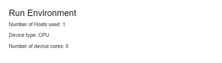
Run Environment provides information on the system where Profiling was conducted. For instance, the environment used for this guide includes one host on a CPU device.
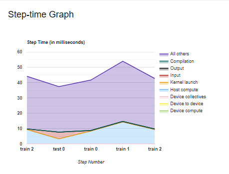
The Step Time graph displays the device step time over all the steps that have been sampled. It shows all the time components included in the performance summary but over different train and test processes.
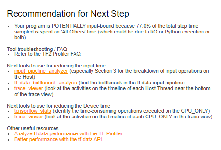
Another vital tool included in the profiler is the recommendations for the next step, which contain suggestions on how to improve your pipeline. The recommendations depend on the kind of model that you have implemented.
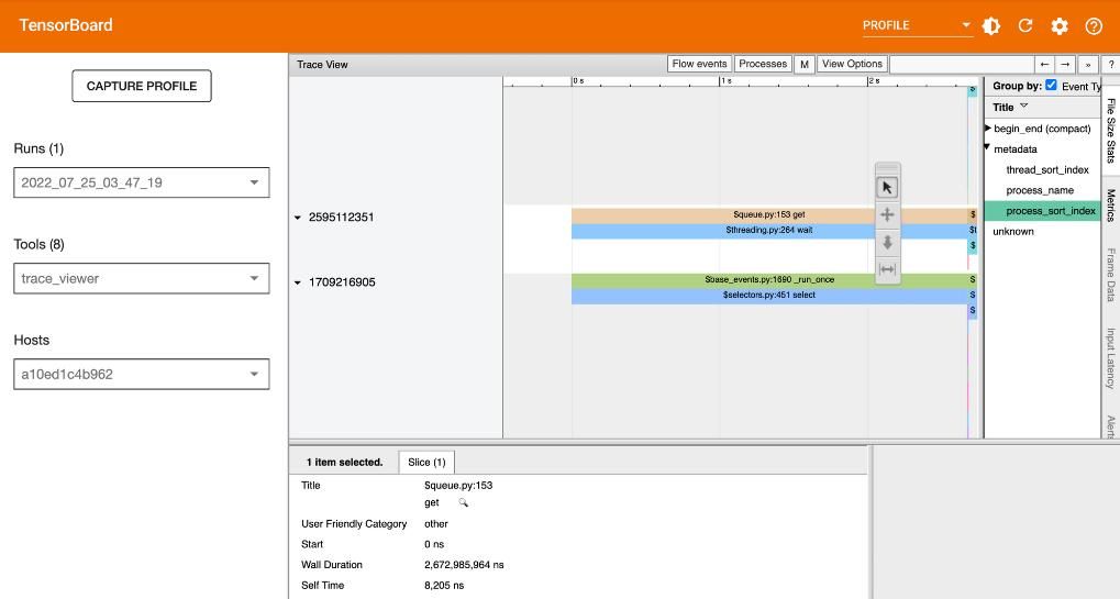
Trace viewer
Selecting Trace Viewer from the Tools drop-down dialogue should return a dashboard similar to the one shown below. It shows a timeline for different events on the GPU or CPU during the profiling process.
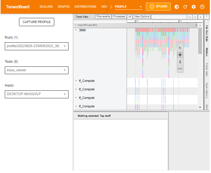
The Trace Viewer is designed such that:
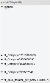
- To the left (vertical grey column), you can see two major sections:
/deviceand/host. This provides information on which TensorFlow op was executed on which device (GPU or CPU resp.). - To the right, the colored bars denote the duration for which the respective TensorFlow ops were executed.
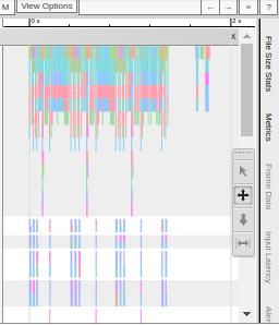
Trace Viewer makes it easy to understand the performance bottlenecks in the input pipeline. Besides, the Trace Viewer provides interactive functionality. Use the keyboard shortcut S. A and D to move to the left and right, respectively. Alternatively, use the navigation widget included in the Trace Viewer window.
To analyze an individual event, use the selection option and click on a TensorFlow Op.
You can use your mouse to select multiple events and analyze the traces based on the selected events or by holding onto the Ctrl key and selecting the desired events.
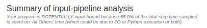
Input pipeline analyzer
The input pipeline analyzer checks the input pipeline and shows whether there is a performance bottleneck in the pipeline. It also tells us whether the model is input bound. The tool contains information related to:
- The Summary of input-pipeline analysis.
- Recommendations for the next step.
- Device-side analysis details.
- Host-side analysis details.
- Input Op statistics.
Summary of input-pipeline analysis includes information on the overall input pipeline. The information shows whether the application is input bound and, if so, to what extent.
Recommendation for the next step provides suggestions on what steps to take next.

Device-side analysis details show the device step-time summary statistics and the graph of time taken during various processes, including:
- Compilation
- Output
- Input
- Kernel launch
- Host compute
- Device collection communication
- Device to device
- Device computation time
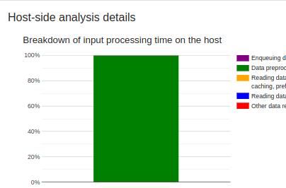
Host-side analysis details provide information on the breakdown of the input processing time on the host. Information contained includes:
- Enqueuing data
- Data preprocessing
- Data reading in both advance and on demand
- other reading data or processing
This guide's processes mainly involved data preprocessing, as shown below.
The Host-side analysis details also include a section for recommendations on what can be done based on the host-side statistics.
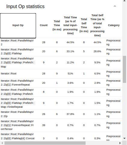
Lastly, the Input Op statistics shows details of various input operations, including:
- Input Op – the name of the underlying TensorFlow input operation.
- Count – number of instances of the operation execution during the profiling session.
- Total Time – the cumulative sum of time spent on each corresponding instance.
- Total Time % – total time spent on an operation as a percentage of the total time spent on processing the input.
- Total Self Time – the cumulative sum of the self-time spent on each instance.
- Total Self Time % – total self-time as a percentage of the total time spent on input processing.
- Category – processing category of the input operation.
mlnuggets newsletter
Join the newsletter to receive the technical deep dives in your inbox.
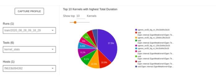
TensorFlow stats
The TensorBoard stats displays the performance of every TensorFlow operation that the host device has executed. The graphs shown might vary depending on the host device and TensorFlow processes. For instance, in this case, there are two pie charts.
The plot to the left shows the distribution of the total self-execution time of each operation on the host, while the last plot shows the distribution of the self-execution time on each operation type on the host.
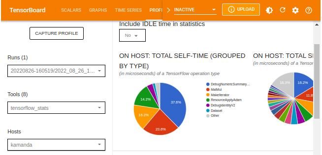
The TensorFlow statistics can be filtered by IDLE time from the dialog box. IDLE time refers to the portion of the total execution time on a device (or host) that is idle.
Other statistics included in the TensorFlow stats dashboard are TensorFlow operations which various details regarding given operations.
GPU kernel stats
If the host device runs with a TPU or GPU kernel, you can view the performance statistics, and the originating operation for each GPU accelerated kernel through kernel_stats windows.
The figure below provides a sample overview of a GPU accelerated kernel.
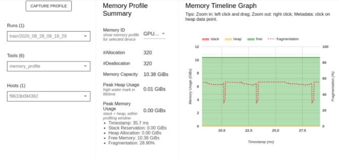
Memory profile page
The Memory profile page tool profiles information on GPU memory usage during TensorFlow Ops. This tool can analyze and debug OOM (Out of Memory) error– raised whenever the GPU’s memory is exhausted.
Components included in the Memory profile page include:
- Memory Profile Summary shows a summary of the memory profile of the TensorFlow application.
- Memory Timeline Graph is a plot of the memory usage in GiBs and the percentage of fragmentation versus time in milliseconds.
- Memory Breakdown Table shows active memory allocations at the point of the highest memory usage in the profiling interval.
mlnuggets newsletter
Join the newsletter to receive the technical deep dives in your inbox.
How to enable debugging on TensorBoard
You can debug the information in the TensorBoard:
- Select particular nodes and debug them.
- Graphically control the execution of the model.
- Visualize the tensors and their values.
To enable debugging, add the following code before the model begins training.
logdir = os.path.join("logs/debugg", datetime.datetime.now().strftime("%Y%m%d-%H%M%S"))

tf.debugging.experimental.enable_dump_debug_info(
    logdir, tensor_debug_mode="FULL_HEALTH", circular_buffer_size=-1
    )
Load TensorBoard.
%tensorboard --logdir logs/debugg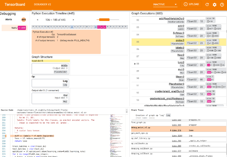
mlnuggets newsletter
Join the newsletter to receive the technical deep dives in your inbox.
Using TensorBoard with deep learning frameworks
TensorBoard allows integration with other machine learning frameworks.
TensorBoard in PyTorch
PyTorch is a popular open-source machine learning framework. You can log PyTorch events using TensorBoard to track loss, RMSE, and accuracy metrics.
First, define a SummaryWriter instance. You will log the events in ./runs/ so delete any prior logs.
import torch #summary instance from torch.utils.tensorboard import
rm -rf ./runs/
SummaryWriter writer = SummaryWriter()
Next, define the data and model, and write the metrics to the SummaryWriter instance.
#install torch
#pip install torch
import torch
#data
x = torch.arange(-5, 5, 0.1).view(-1, 1)
y = -5 * x + 0.1 * torch.randn(x.size())
#model
model = torch.nn.Linear(1, 1)
criterion = torch.nn.MSELoss()
optimizer = torch.optim.SGD(model.parameters(), lr = 0.1)

def train_model(iter):
    for epoch in range(iter):
        y1 = model(x)
        loss = criterion(y1, y)
        writer.add_scalar("Loss/train", loss, epoch)
        optimizer.zero_grad()
        loss.backward()
        optimizer.step()

train_model(10)
writer.flush()
#close writer
writer.close()
To avoid cluttering, especially in cases where you have a large sample, you can arrange the results in the SummaryWriter instance as shown below.
from torch.utils.tensorboard import SummaryWriter
import numpy as np
writer = SummaryWriter()
for n_iter in range(100):
    writer.add_scalar('Loss/train', np.random.random(), n_iter)
    writer.add_scalar('Loss/test', np.random.random(), n_iter)
    writer.add_scalar('Accuracy/train', np.random.random(), n_iter)
    writer.add_scalar('Accuracy/test', np.random.random(), n_iter)
Load TensorBoard.
%tensorboard --logdir=runs
TensorBoard in Keras
To add Keras models to the TensorBoard, first, create a Keras callback object of TensorBoard whose logs will be saved in the experiment folder inside the folder containing the main logs.
tb_callback = tf.keras.callbacks.TensorBoard(log_dir="logs/experiment", histogram_freq=1)
model = create_model()

model.fit(X_train, y_train, epochs=10, callbacks=[tb_callback])
Now run and visualize the Keras model in TensorBoard.
%tensorboard --logdir logs/experiment
TensorBoard in XGBoost
XGBoost is another popular ML package used for classification and regression problems. To log events from XGBoost modeling, you need the tensorboardX package which can be installed using pip install tensorboardX. To work with XgBoost, install the package using:
conda install -c anaconda py-xgboost from your command prompt or !conda install -c anaconda py-xgboost in Google Colab notebook.
This example logs the events for an XGBoost model trained on the popular Ames housing dataset.
Remove prior logs rm -rf ./runs/ and define the XGBoost model.
import datetime
#conda install -c anaconda py-xgboost
import xgboost as xgb
import os
#set some xgboost attributes that miss in version 1.6.x
new_attrs = ['grow_policy', 'max_bin', 'eval_metric', 'callbacks', 'early_stopping_rounds', 'max_cat_to_onehot', 'max_leaves', 'sampling_method']

for attr in new_attrs:
    setattr(xgb, attr, None)
from tensorboardX import SummaryWriter

from sklearn.model_selection import train_test_split


class TensorBoardCallback(xgb.callback.TrainingCallback):
    '''
    Run experiments while scoring the model and saving the error to train or test folders
    '''
    def __init__(self, experiment: str = None, data_name: str = None):
        self.experiment = experiment or "logs"
        self.data_name = data_name or "test"
        self.datetime_ = datetime.datetime.now().strftime("%Y%m%d-%H%M%S")
        #save the logs to the 'run/' folder
        self.log_dir = f"runs/{self.experiment}/{self.datetime_}"
        self.train_writer = SummaryWriter(log_dir=os.path.join(self.log_dir, "train/"))
        if self.data_name:
            self.test_writer = SummaryWriter(
                log_dir=os.path.join(self.log_dir, f"{self.data_name}/")
            )

    def after_iteration(
        self, model, epoch: int, evals_log: xgb.callback.TrainingCallback.EvalsLog
    ) -> bool:
        if not evals_log:
            return False

        for data, metric in evals_log.items():
            for metric_name, log in metric.items():
                score = log[-1][0] if isinstance(log[-1], tuple) else log[-1]
                if data == "train":
                    self.train_writer.add_scalar(metric_name, score, epoch)
                else:
                    self.test_writer.add_scalar(metric_name, score, epoch)

        return False


from sklearn.datasets import fetch_openml
X, y =  fetch_openml(name="house_prices", return_X_y=True)
#subset numerical variables
numerics = ['int16', 'int32', 'int64', 'float16', 'float32', 'float64']
X = X.select_dtypes(include=numerics)
#subset the data to train and test
X_train, X_test, y_train, y_test = train_test_split(X, y, test_size=0.2, random_state=100)

dtrain = xgb.DMatrix(X_train, label=y_train, enable_categorical = True)
dtest = xgb.DMatrix(X_test, label=y_test, enable_categorical = True)

params = {'objective':'reg:squarederror', 'eval_metric': 'rmse'}

bst = xgb.train(params, dtrain, num_boost_round=100, evals=[(dtrain, 'train'), (dtest, 'test')],
        callbacks=[TensorBoardCallback(experiment='exp_1', data_name='test')])
Next, load the TensorBoard using the logs saved to SummaryWriter.
%tensorboard --logdir runs/
mlnuggets newsletter
Join the newsletter to receive the technical deep dives in your inbox.
TensorBoard in JAX and Flax
You can log evaluation metrics when using JAX during model training, use TensorBoard to profile JAX programs using the jax.profiler.start_trace() and jax.profiler.stop_trace() to start and stop JAX tracing, respectively.
from torch.utils.tensorboard import SummaryWriter
import torchvision.transforms.functional as F
log_folder = "runs"

writer = SummaryWriter(logdir)
for epoch in range(1, num_epochs + 1):
    train_state, train_metrics = train_one_epoch(state, train_loader)
    training_loss.append(train_metrics['loss'])
    training_accuracy.append(train_metrics['accuracy'])
    print(f"Train epoch: {epoch}, loss: {train_metrics['loss']}, accuracy: {train_metrics['accuracy'] * 100}")

    test_metrics = evaluate_model(train_state, test_images, test_labels)
    testing_loss.append(test_metrics['loss'])
    testing_accuracy.append(test_metrics['accuracy'])

    writer.add_scalar('Loss/train', train_metrics['loss'], epoch)
    writer.add_scalar('Loss/test', test_metrics['loss'], epoch)

    writer.add_scalar('Accuracy/train', train_metrics['accuracy'], epoch)
    writer.add_scalar('Accuracy/test', test_metrics['accuracy'], epoch)

    print(f"Test epoch: {epoch}, loss: {test_metrics['loss']}, accuracy: {test_metrics['accuracy'] * 100}")
The figure below shows a manual sample profiling of JAX.
Read more: How to use TensorBoard in JAX & Flax
Download TensorBoard data as Pandas DataFrame
After you have finished modeling, you might be interested in conducting post-hoc analyses and creating custom visualizations based on log data. TensorBoard allows you to access your log data using data.experimental.ExperimentFromDev() function.
Consider the Iris classification problem. You can access the data for a given experiment using:
import tensorboard as tb

experiment_id = "c1KCv3X3QvGwaXfgX1c4tg"
experiment = tb.data.experimental.ExperimentFromDev(experiment_id)
df = experiment.get_scalars()
df.head()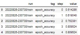
You can also obtain the DataFrame as a wide format since, in the experiment, the two tags (epoch_loss and epoch_accuracy) are present at the same set of steps in each run.
try:
    experiment_id = "c1KCv3X3QvGwaXfgX1c4tg"
    experiment = tb.data.experimental.ExperimentFromDev(experiment_id)
    df = experiment.get_scalars()

    df_wide = experiment.get_scalars(pivot=True)
    display(df_wide.head())
except:
    print("There is only a single tag")
    df_wide = experiment.get_scalars(pivot=False)
    display(df_wide.head())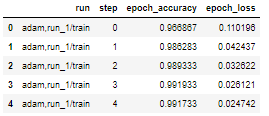
Finally, you can save the Pandas DataFrame as a CSV file.
#path
import pandas as pd
csv_path = 'tensor_experiment_1.csv'
df_wide.to_csv(csv_path, index=False)
df_wide_roundtrip = pd.read_csv(csv_path)
pd.testing.assert_frame_equal(df_wide_roundtrip, df_wide)
You can now visualize the data using a visualization package such as Matplotlib.
mlnuggets newsletter
Join the newsletter to receive the technical deep dives in your inbox.
Tensorboard.dev
With TensorBoard, you can easily host, track, and share ML experiments. All you need to do is upload logs to TensorBoard.dev. Sharing logs is possible in Google Colab or from the command prompt.
In your working directory, open the command prompt and run:
tensorboard dev upload --logdir logs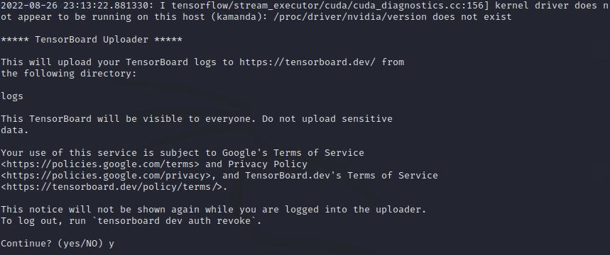
On Google Colab notebook:
%tensorboard dev upload --logdir logsOn Jupyter Notebook:
!tensorboard dev upload --logdir logs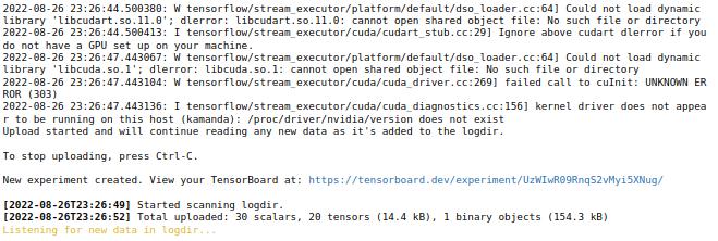
You will be prompted to continue with the upload by entering y/yes; otherwise, abort the operation. After supplying Yes, an authorization window for www.google.com will be opened for you to complete the process. Upon successful completion, a unique link for the experiment will be created. The following link shows an example of an uploaded TensorBoard.
To stop uploading, interrupt the execution in Jupyter and Google Colab notebooks or press Ctrl-C if you are using the command prompt.
Limitations of using TensorBoard
TensorBoard has its share of limitations. Some of the limitations of TensorBoard include:
- Lacks private hosting. All experiments shared using Tensorboard.dev are public. Be keen not to upload sensitive information to TensorBoard.dev.
- TensorBoard is limited to specific data formats limiting the logging and visualization of other data formats such as audio/video or custom HTML.
- Lack of user and workspace management features often necessary for larger organizations.
- Scalability issues. TensorBoard starts getting performance issues as the number of runs increases.
- Does not offer functionality for team collaboration which disadvantages users who work on ML products as a team.
Final thoughts
The process of machine learning engineering, which every data scientist interacts with from time to time, requires extensive modeling using different frameworks to optimize the underlying models' predictive ability. However, the process of model optimization, debugging, and deployment can present its fair share of challenges. Tools like TensorBoard provide developers with resources to build better machine learning models and produce quality results with less effort.
From setting up TensorBoard to debugging and visualizing logs from other libraries, this guide delves into the functionality of TensorBoard in visualizing the machine learning modeling process.
TensorFlow Resources
- Object detection with TensorFlow 2 Object detection API
- How to train deep learning models on Apple Silicon GPU
- How to build CNN in TensorFlow(examples, code, and notebooks)
- How to build artificial neural networks with Keras and TensorFlow
- Custom training loops in Keras and TensorFlow
- Flax vs. TensorFlow
- How to build TensorFlow models with the Keras Functional API
- TensorFlow Recurrent Neural Networks (Complete guide with examples and code)
Whenever you're ready, there is 2 way I can help you:
If you're looking for a way to build a career while writing about data science and machine learning, I'd recommend starting with an affordable ebook:
→ Writing for Data Scientists: The exact path I followed to get technical work that pays between $250-$500 from machine learning companies such as Comet, Neptune, cnvrg, Paperspace, Layer, Neural Magic, Determined, Activeloop, and many more. Get your copy.
→ Data Science and Machine Learning Ebook: I offer numerous free and paid data science and machine learning ebooks to help you in your data science career. Check them out.