
Decision Trees and Random Forests(Building and optimizing decision tree and random forest models)

In the modern world, so much data is present on the internet. Organizations need efficient and rigorous algorithms to handle these huge chunks of data, make practical analyses, and provide appropriate decisions relevant to maximizing their profits and market presence. There are such algorithms commonly used today for decision-making processes. They are:
- Decision Trees.
- Random Forests.
What is a Decision Tree?
Decision trees, also known as Classification and Regression Trees (CART), are supervised machine-learning algorithms for classification and regression problems. A decision tree builds its model in a flowchart-like tree structure, where decisions are made from a bunch of "if-then-else" statements.
Below is a pictorial representation of what a decision tree will look like:
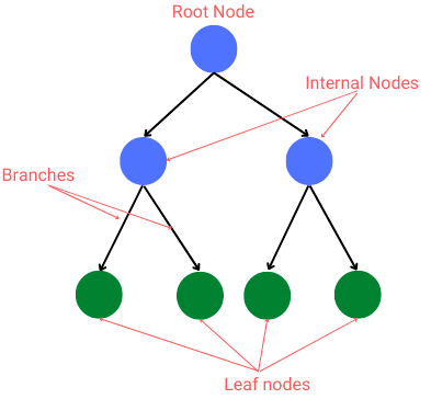
From the diagram, we take note of some terminologies:
- Root node: first node in the tree. This node has no incoming branches.
- Internal nodes: these are the decision nodes.
- Branches: they are arrows connecting nodes. They represent the decision-making steps.
- Leaf Nodes: these nodes represent all the possible outcomes from a dataset.
Decision trees allow continuous data splitting based on given parameters until a final decision is reached. They start with a single node which then branches into possible outcomes. The possible outcomes break into additional nodes, branching into more possible outcomes hence the tree structure.
For instance, when planning a game, we may want to decide whether the match will take place depending on data of parameters like weather, humidity, and wind. The resulting tree would be something like this:
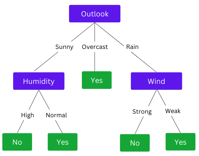
The example shows how a decision tree splits into different data points until a final decision is achieved.
Read our Entropy, information gain, and Gini impurity tutorial to know how a decision tree:
- Decides on the first node from where the splitting begins.
- Creates and splits on internal nodes.
- Decides to stop splitting on a particular node.
Types of Decision Trees
Decision trees are categorized based on the type of target variable. They can be of two types:
- Continuous Variable Decision tree: Decision tree where the target variable is continuous. For instance, we can build a decision tree to decide a person's age based on DNA methylation levels.
- Categorical Variable Decision tree: Decision tree where the target variable is categorical. A category can be a yes or no, meaning that the decision falls under only one category for every stage.
Decision Tree algorithms
Algorithms used in decision trees are also based on the target variable type. They include:
ID3(Iterative Dichotomiser)
This algorithm uses entropy and information gain to decide on the split points. It uses a greedy search approach to select the best attribute to split the dataset on each iteration.
C4.5 algorithm
It uses information gain to evaluate split points. It extends Quinlan’s earlier ID3 algorithm and is often referred to as a statistical classifier.
CART(Classification and Regression Trees)
This is the most well-established and used algorithm.
- They are a non-parametric decision tree learning technique.
- They produce classification or regression trees based on whether the dependent variable is categorical or numeric.
- They use the Gini impurity to decide on split points.
- We can also use this algorithm to detect anomalies and outliers.
Splitting criteria for Decision Trees
The main idea of a decision tree is to identify features that contain adequate information about a target feature and then split the dataset along with their values. The search for the most informative attribute creates a decision tree until we get pure leaf nodes.
There are various criteria used by decision trees to select the best attribute for splitting at each node. they include:
- Entropy
- Information gain
- Gini impurity
Learn more on these criteria in our Entropy, information gain, and Gini impurity tutorial.
Assumptions of Decision Trees
A decision tree does not make assumptions about the training data or prediction residues since it uses a non-statistical approach. However, there are some assumptions that we make when building decision trees:
- As we begin building the tree, the whole training set is assumed to be the root.
- The preferred feature values are categorical. If we have continuous values, they are discretized before the model is built.
- Records are distributed recursively based on attribute values.
- The order of placing attributes as the root or internal nodes is done using a statistical approach.
What is a Random Forest?
It is easy to understand and make meaning of decision tree algorithms. However, sometimes producing a single tree is not adequate for effective results. This is where random forests suffice.
A random forest is an ensemble method called Bootstrap Aggregation or bagging that uses multiple decision trees to make decisions. As its name suggests, it is actually a "forest" of decision trees.
We call it a "random" forest since it:
- Randomly samples the training dataset to build a tree.
- Generates a random subset of features to calculate the output for splitting nodes.
General differences between a Decision Tree and Random Forest
Decision trees and random forests have significant differences. The table below gives a side-by-side comparison based on various issues.
| Issue | Decision Tree | Random Forest |
|---|---|---|
| Time | Less time to run | More time to run |
| Speed | It's fast | Quite slow |
| Overfitting | Most likely to overfit | It uses several decision trees and is thus less likely to overfit |
| Interpretation | Easy to interpret | Complex to interpret |
| Visualization | Easy to visualize | Complex to visualize |
| Accuracy | Less accurate | More accurate results |
| Computation | Low computation | Consumes more computation |
Building a Decision Tree and Random Forest
We will build a Decision tree and random forest models using Python's Scikit-learn library. We will compare the two models' results and determine which performs best.
Let's first prepare the dataset.
The dataset
We will use the Red wine quality dataset from Kaggle. The dataset has 12 features from which we will build a decision tree model and a random forest to decide whether a particular wine is good(1) or not (0).
Let's have a look at the dataset.
import pandas as pd

data = pd.read_csv('winequality-red.csv')
print('Shape: ', data.shape)
data.head()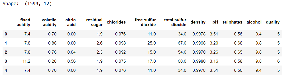
# check frequency of the unique values in quality column
df['quality'].value_counts()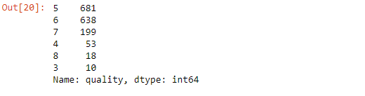
Let's label the quality column with bad and good labels where a value less than 6 is considered bad, and a value above 6 is good quality.
# label the quality column

bins = (2, 6, 8) # 2-6 = bad quality, 6-8=good quality
groups = ['bad', 'good']
data['quality'] = pd.cut(data['quality'], bins = bins, labels = groups)
data.head(10)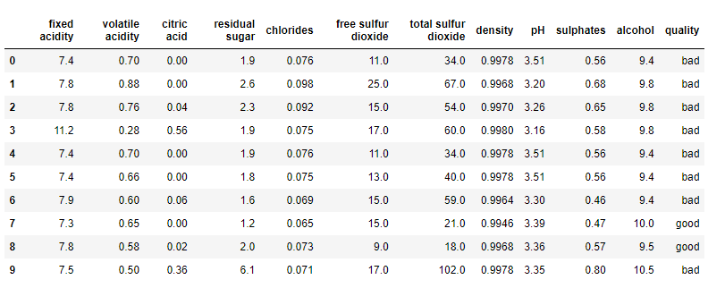
Let's now encode the quality column from categorical to numerical form necessary for building the model.
# encode the 'quality' column

quality_label = LabelEncoder()
data['quality'] = quality_label.fit_transform(data['quality'])
data['quality'].value_counts()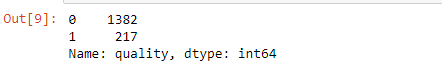
df.head(10)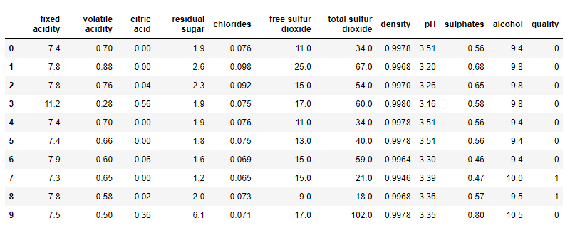
Visualize the quality column count.
import seaborn as sns
sns.countplot(x='quality',data=data)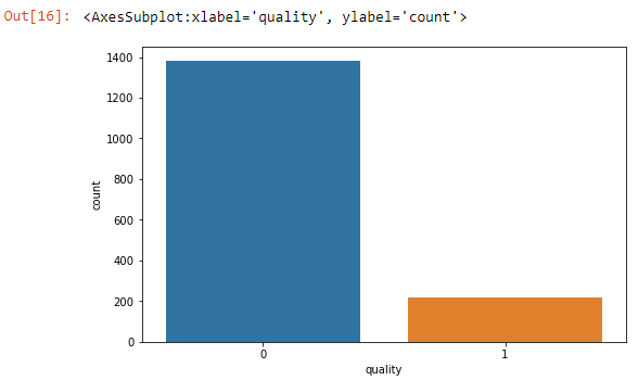
Creating the train and test sets
Let's first divide the dataset into independent and dependent variables. The 'quality' feature will serve as the target variable.
X = data.drop('quality', axis=1)
y = data['quality']
Split the dataset into training and test set.
from sklearn.model_selection import train_test_split

X_train, X_test, y_train, y_test = train_test_split(X, y, test_size=0.30, random_state=42)
Building a Decision Tree model with sklearn
Now it's time to build a decision tree. Scikit-learn provides a sklearn.tree.DecisionTreeClassifier class. We will consider some of the following parameters:
criterion- measures the quality of a split. The criteria supported are Gini and entropy for information gain.splitter- strategy for choosing a split at each node. Supports 'best' and 'random' strategies.max_depth- maximum depth of the tree. The deeper the tree, the more complex the decision rules, and the fitter the model.random_state- controls the randomness of splitting.min_samples_split- The minimum number of samples required to split an internal node.min_samples_leaf- The minimum number of samples required to be at a leaf node.max_leaf_nodes- Grow a tree withmax_leaf_nodesin best-first fashion. Best nodes are defined as relative reduction in impurity. If None, then an unlimited number of leaf nodes.
The steps we take are:
- Import the DecisionTreeClassifier class.
- Instantiate the classifier model.
- Fit the model.
- Predict.
- Evaluate model performance.
from sklearn.tree import DecisionTreeClassifier

clf = DecisionTreeClassifier(random_state=42) # instantiate the model
clf = clf.fit(X_train, y_train) # fit the model

# making predictions
y_pred = clf.predict(X_test) # Test the prediction accurracy of the model
result = pd.DataFrame({'Actual' : y_test, 'Predicted' : y_pred})
pd.concat([result.head(), result.tail()]) # display df of acutal and predicted(head and tail)
Check the model's accuracy.
from sklearn.metrics import accuracy_score
print('Testing Set Evaluation Accuracy: ',accuracy_score(y_test,y_pred))

# Testing Set Evaluation Accuracy:  0.8604166666666667
Confusion matrix.
from sklearn.metrics import confusion_matrix

cf_matrix = confusion_matrix(y_test, y_pred) # generate confusion matrix
sns.heatmap(pd.DataFrame(cf_matrix), annot=True, cmap='RdYlBu', linewidth=.5, fmt='g', cbar=False)
plt.title('Confusion matrix', y=1.1)
plt.ylabel('Actual label')
plt.xlabel('Predicted label')
cf_matrix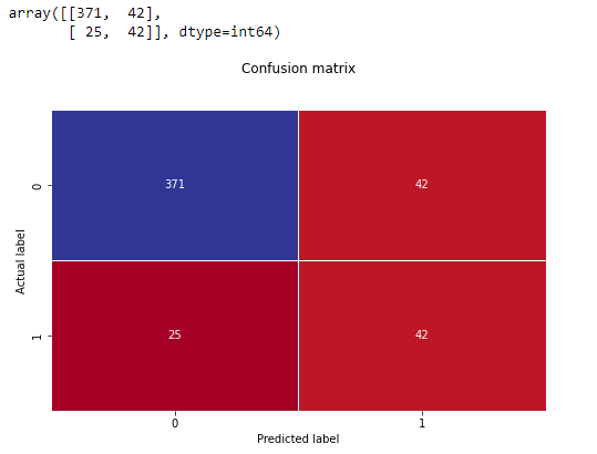
So we have 67 wines classified as false.
Classification report:
from sklearn.metrics import classification_report

target_names = ['Bad Quality', 'Good Quality']
pd.DataFrame(classification_report(y_test, y_pred,target_names=target_names, output_dict=True))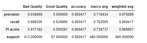
Before we can visualize the Decision tree we've just built, we have a chance to improve the model's performance through hyperparameter tuning.
In hyperparameter tuning, we specify possible parameters best for optimizing the model's performance. Since it is impossible to manually know the optimal parameters for our model, we will automate this using sklearn.model_selection.GridSearchCV class.
Let's look at how we can perform this on a Decision Tree Classifier.
Hyperparameter tuning on Decision Tree Classifier
We will import the GridSearchCV class from sklearn and then pass predefined values for hyperparameters to it.
from sklearn.model_selection import GridSearchCV

# defining parameters
param_grid = {
    "criterion":("gini", "entropy"),
    "splitter":("best", "random"),
    "max_depth":(list(range(1, 15))),
    "min_samples_split":[2, 3, 4, 6, 8],
    "min_samples_leaf":list(range(1, 15)),
}
# training model on the define params with GridSearchCV
clf_tree = DecisionTreeClassifier()
tree_cv = GridSearchCV(clf_tree, param_grid,scoring="accuracy",
                       n_jobs=-1, verbose=1, cv=3)

tree_cv.fit(X_train, y_train)
predictions = tree_cv.predict(X_test)
optimal_params = tree_cv.best_params_
print(f"\nOptimal paramters: ({optimal_params})")

print("\n====BEST MODEL SCORE====")
print('Best model score: ', tree_cv.best_score_)

print("\n====CLASSIFICATION REPORT====")
target_names = ['Bad Quality', 'Good Quality']
pd.DataFrame(classification_report(y_test,
                                   predictions,
                                   target_names=target_names,
                                   output_dict=True))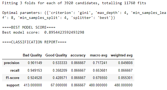
So the most accurate tree should have the above optimal parameter values, for instance, a max-depth of 4.
Visualizing Decision Tree
We can use at least 4 methods to visualize a decision tree:
- Printing a text representation of the tree with sklearn.tree.export_text method: exports decision tree to a text representation, especially for applications with no user interface.
- Plotting with sklearn.tree.plot_tree method: requires matplotlib.
- Plotting with sklearn.tree.export_graphviz: requires Pythongraphviz module.
- Plotting with dtreeviz package: will require dtreeviz and graphviz.
We will visualize our decision tree with the sklearn.tree.export_graphviz method. For it to work, you will need to:
- Install Graphviz.
conda install python-graphviz- Install pydotplus.
pip install pydotplusImport the required modules and visualize.
from sklearn.tree import export_graphviz
from six import StringIO
from IPython.display import Image

dot_data = StringIO()
export_graphviz(clf, out_file=dot_data, feature_names=features, filled=True)
graph = pydotplus.graph_from_dot_data(dot_data.getvalue())
Image(graph.create_png())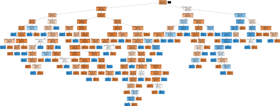
Interpreting this kind of tree is quite a hustle. There are very many rules applied. The next section will examine how we can prune the tree to reduce its complexity and control overfitting.
Pruning Decision Trees
In most cases, decision trees are prone to overfitting. A decision tree will overfit when allowed to split on nodes until all leaves are pure or until all leaves contain less than min_samples_split samples. That is, allowing it to go to its max-depth.
Allowing a decision tree to go to its maximum depth results in a complex tree, as in our example above.
Pruning can be classified into:
- Pre-pruning
- Post-pruning
Pre-pruning
Pre-pruning can also be termed "early stopping." Here we try to stop the tree from splitting to its maximum depth. Remember:
- The decision tree we have created above is complex and not easily explainable.
- We performed hyperparameter tuning, where we got the optimal parameter values.
To simplify the model, we can retrain it with the values from hyperparameter tuning, get its accuracy and visualize the tree again.
clf = DecisionTreeClassifier(criterion='gini',
                             max_depth=4,
                             splitter='best',
                             min_samples_leaf=8,
                             min_samples_split=4,
                             random_state=42
                            )

clf = clf.fit(X_train, y_train)
print('Testing Set Evaluation Accuracy: ',
      accuracy_score(y_test,clf.predict(X_test)))

# Testing Set Evaluation Accuracy:  0.8666666666666667
You can see that our model accuracy has a slight improvement. Let's visualize:
# visualizing
dot_data = StringIO()
export_graphviz(clf, out_file=dot_data, feature_names=features, filled=True)
graph = pydotplus.graph_from_dot_data(dot_data.getvalue())
Image(graph.create_png())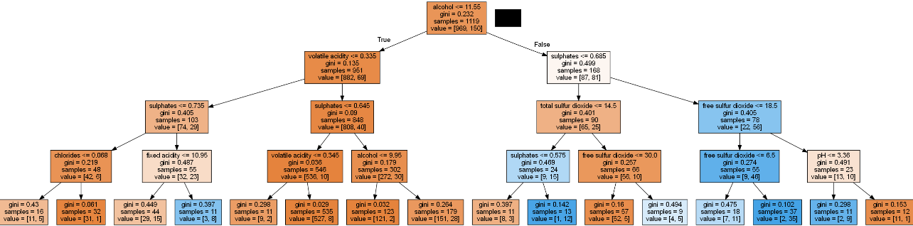
We can also observe that the rules have been reduced, and the model is a little easy to interpret.
Post-pruning
In post-pruning, we allow the tree to train perfectly on the training set and then prune it. The DecisionTreeClassifier has a parameter named ccp_alpha. This parameter is called the cost-complexity parameter(See the math behind it).
Generally, the cost-complexity printing recursively finds the node with the "weakest link." The weakest link is characterized by an effective alpha, where the nodes with the smallest effective alpha are pruned first.
Let's see how it's done.
path = clf.cost_complexity_pruning_path(X_train, y_train)
ccp_alphas, impurities = path.ccp_alphas, path.impurities
To get an idea of what values of ccp_alpha parameter could be viable, we use the cost_complexity_pruning_path which gives us the alphas and the corresponding total leaf impurities at each step of the pruning process.
ccp_alphas variable stores the weak points with respect to each node in the form of a list.
ccp_alphas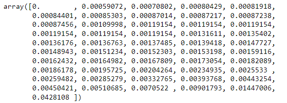
We will train our decision tree model using these alpha values.
# grid search to find the optimal value for alpha from the ccp_alphas list

clf_tree = DecisionTreeClassifier(random_state=42)
ccp_alpha_grid_search = GridSearchCV(clf_tree, param_grid=({"ccp_alpha":[alpha for alpha in ccp_alphas]}))

ccp_alpha_grid_search.fit(X_train, y_train) # # train model
# find the best parameter value
print('Best parameter:' , ccp_alpha_grid_search.best_params_)
We see that the best decision tree will be generated by a ccp_alpha of value 0.009017930023689974.
We again visualize the pruned decision tree and get a very simple and easy-to-understand tree.
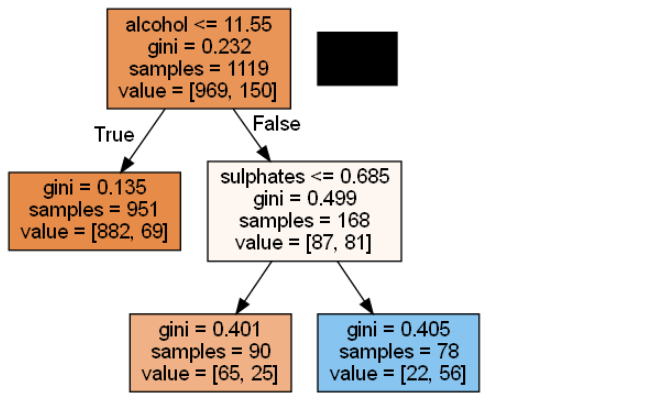
As the alpha values increase, more of the tree is pruned, increasing the total impurity of its leaves and, thus, a tree that generalizes better.
Building a Random Forest model with Sklearn
A random forest fits several decision tree classifiers on various sub-samples of the dataset. It uses averaging to improve predictive accuracy and control over-fitting. Random trees achieve a higher classification accuracy than decision trees.
Scikit-learn provides a sklearn.tree.RandomForestClassifier class. The class has some of the following parameters:
n_estimators: The number of trees in the forest.criterion: The function to measure the quality of a split. Supported criteria are "gini" for the Gini impurity and "entropy" for the information gain.max_depth: The maximum depth of the tree.min_samples_split: The minimum number of samples required to split an internal node.min_samples_leaf: The minimum number of samples required to be at a leaf node.bootstrap: Whether bootstrap samples are used when building trees. If False, the whole dataset is used to build each tree.oob_score: Whether to use out-of-bag samples to estimate the generalization accuracy.
Before we proceed, let's create a function to avoid too much repetition.
def eval_model_score(clf, X_train, y_train, X_test, y_test):
    y_pred = clf.predict(X_test)
    print('Testing Set Evaluation Accuracy: ',accuracy_score(y_test,y_pred))
    print("\n====CONFUSION MATRIX====\n")
    print(confusion_matrix(y_test, y_pred)) # generate confusion matrix
    print("\n====CLASSIFICATION REPORT====")
    target_names = ['Bad Quality', 'Good Quality']
    clf_report = pd.DataFrame(classification_report(y_test, y_pred,                                                    target_names=target_names,
                                                    output_dict=True
                                                    ))
    print(clf_report)
Let's dive in!
from sklearn.ensemble import RandomForestClassifier

rf_clf = RandomForestClassifier(random_state=42)
rf_clf.fit(X_train, y_train)
eval_model_score(rf_clf, X_train, y_train, X_test, y_test)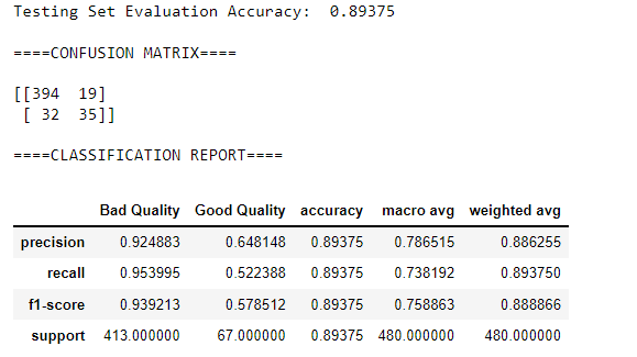
Straight away, we can observe that the random forest classifier gives more accuracy than the decision tree classifier. Later on, we will explain why random forests perform better.
Hyperparameter tuning on Random Tree Classifier
We can find the best parameters to improve our model's performance using sklearn.model_selection.RandomizedSearchCV class.
The key difference between the RandomSearchCV and GridSearchCV is that while GridSearchCV tests all parameters and selects the best, RandomSearchCV does not test all parameters but instead searches randomly.
RandomSearchCV also has the n_iter parameter that helps specify the number of parameter values we want to test.
from sklearn.model_selection import RandomizedSearchCV

# Provide hyperparameter grid for a random search
n_estimators = [int(x) for x in np.linspace(start=200, stop=2000, num=10)]
max_features = ['auto', 'sqrt']
max_depth = [int(x) for x in np.linspace(10, 120, num=12)]
max_depth.append(None)
min_samples_split = [2, 5, 10]
min_samples_leaf = [1, 2, 4]
bootstrap = [True, False]

random_grid = {'n_estimators': n_estimators, 'max_features': max_features,
               'max_depth': max_depth, 'min_samples_split': min_samples_split,
               'min_samples_leaf': min_samples_leaf, 'bootstrap': bootstrap}

rf_cv = RandomizedSearchCV(estimator=rf_clf, scoring='accuracy',
                           param_distributions=random_grid,
                           n_iter=50, cv=5, verbose=2,
                           random_state=42, n_jobs=-1
                          )

rf_cv.fit(X_train, y_train)
rf_best_params = rf_cv.best_params_
print(f"Best paramters: {rf_best_params})")

eval_model_score(rf_clf, X_train, y_train, X_test, y_test)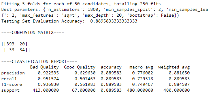
Train the model with the tuned parameters.
rf_clf = RandomForestClassifier(**rf_best_params) # pass the best parameters as **kwargs
rf_clf.fit(X_train, y_train)
eval_model_score(rf_clf, X_train, y_train, X_test, y_test)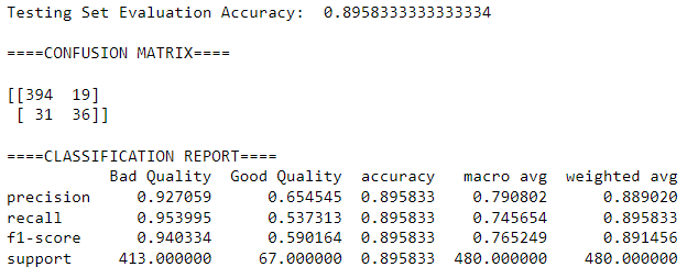
Why Random Forest performed better than Decision Tree
Unlike random forests, decision trees give high importance to a specific set of features. A random forest randomly chooses features during the training process; thus, it does not rely on any particular set of features.
The random nature of feature selection by random forest makes it generalize the data in a more excellent which makes it more accurate than a decision tree.
So should you choose to use a Decision Tree or Random Forest?
The choice depends on the dataset you are working on or the interpretability concerns.
Random forest is ideal for large datasets, and interpretability is not a major concern. It is easier to understand and interpret decision trees than random forests since a random forest combines several decision trees, thus making it a little complex to understand.
A random forest also has a higher training time than a single decision tree, and this is because as the number of trees increases in a random forest, so is the time taken to train each of them.
Decision trees make it easier to quickly and understandably build, even for anyone with little knowledge about them.
Final thoughts
In this article, we have gained excellent knowledge of decision trees and random forests. We covered:
- What a decision tree and a random forest are.
- Parts of a decision tree.
- Examples of decision tree algorithms.
- How to build both models.
- Hyperparameter tuning with cross-validation using
GridSearchCVandRandomizedSearchCV.
... to mention a few.
You may have noticed that we have dealt with a classification problem for this article. Decision trees can also be done for regression problems, but we shall cover that in a future article.
The Complete Data Science and Machine Learning Bootcamp on Udemy is a great next step if you want to keep exploring the data science and machine learning field.
Follow us on LinkedIn, Twitter, and GitHub, and subscribe to our blog, so you don't miss a new issue.