Entropy, information gain, and Gini impurity(Decision tree splitting criteria)

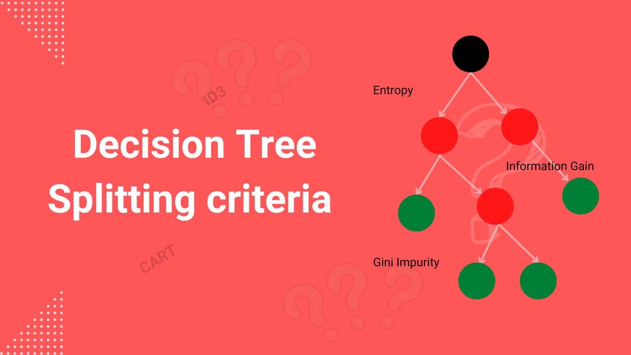
Decision trees are supervised machine-learning models used to solve classification and regression problems. They help to make decisions by breaking down a problem with a bunch of if-else-then-like evaluations that result in a tree-like structure.

For quality and viable decisions to be made, a decision tree builds itself by splitting various features that give the best information about the target feature till a pure final decision is archived.

This article will discuss three common splitting criteria used in decision tree building:

• Entropy
• Information gain
• Gini impurity

Entropy

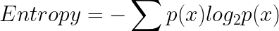
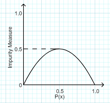
Entropy measures data points' degree of impurity, uncertainty, or surprise. It ranges between 0 and 1.

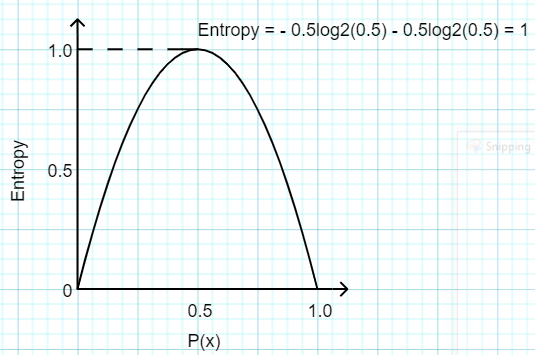
We can see that the entropy is 0 when the probability is o or 1. We get a maximum entropy of 1 when the probability is 0.5, which means that the data is perfectly randomized.

To understand entropy, let's familiarize ourselves with the concept of surprise. Surprise, by definition, is an unexpected event.

Suppose we had three baskets with random colored balls:

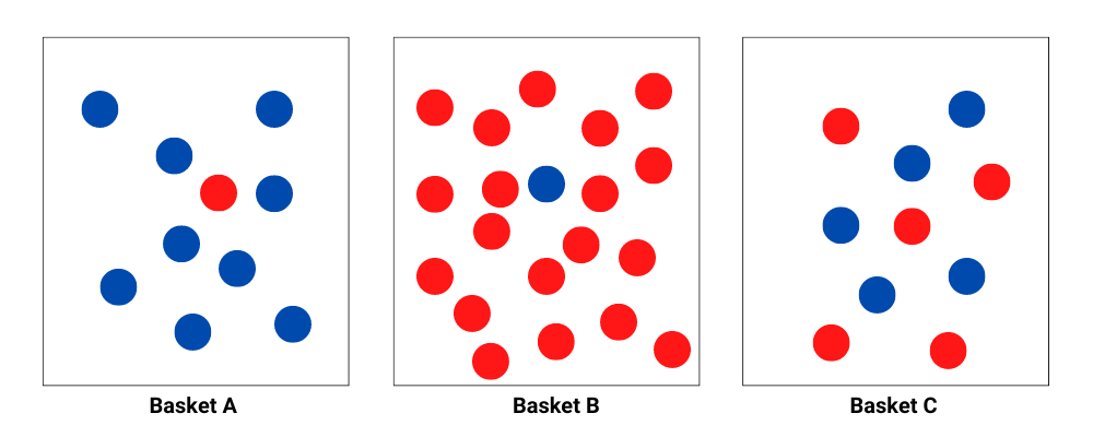
Each basket has a varying number of red and blue balls. Suppose we decided to pick a random ball from each basket. We will notice that:

• From Basket A, the probability of picking a blue ball is higher than that of picking a red ball. We would be very surprised if we picked a red ball.
• From Basket B, the probability of picking a red ball is higher than that of picking a blue ball. We would be relatively surprised if we picked a blue ball.
• From Basket C, the probability of picking either a red or blue ball is equal. Regardless of what ball we picked, we would be equally surprised.

The results show that surprise is inversely related to probability(p(x)). That is, for instance, from Basket A, when the probability of picking a red ball is low, the surprise is high (1/p(x)).

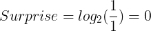
However, we can not use the inverse of probability to calculate the surprise. For instance, let's say we decided to pick balls from basket A three times.

If we picked blue balls and never picked a red one each time we picked, then it would be relatively correct to say that the probability of picking a red ball would always be 0 and that of picking a blue ball 1  for each round we decided to pick. That means the surprise of picking a blue ball should be 0 for each round. But the inverse of the probability of picking a blue ball is 1 1/1 = 1.

Since we have found out that we can not use the inverse of probability to calculate the surprise, we introduce log to the inverse of probability:

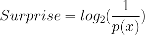
Thus the surprise of picking a blue ball from basket A the given number of times would be 0, just as expected:

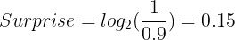
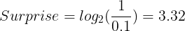
Now with the knowledge of expected values, we can try to calculate the surprise of picking a blue ball and a red ball from Basket A. Since we already know that there's a 0.1 chance that we would pick a red ball and a 0.9 chance of picking a blue ball, we would have the following:

Surprise for picking a blue ball:

Surprise for picking a red ball:

Entropy is now the expected value of surprise. So every time we pick a ball from basket A, we expect a certain amount of surprise. That is:

Now from this, we can derive the formula for Entropy:

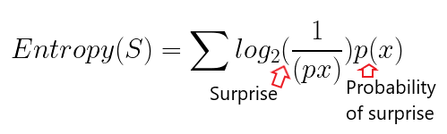
From the equation above, we can get the standard equation for Entropy:

Having understood what entropy is and its formula, let's calculate the entropy of the balls from each basket in our example above:

Entropy in basket A:

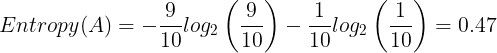
import math

entropy_A = -(9/10) * math.log2(9/10) - (1/10) * math.log2(1/10)
entropy_A
# 0.4689955935892812

Entropy in basket B:

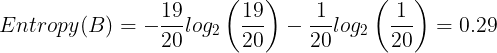
entropy_B = -(19/20) * math.log2(19/20) - (1/20) * math.log2(1/20)
entropy_B
# 0.28639695711595625

Entropy in basket C:

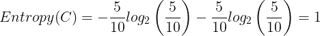
entropy_C = -(5/10) * math.log2(5/10) - (5/10) * math.log2(5/10)
entropy_C
# 1.0

The higher the entropy, the less pure the dataset or, the higher the level of disorder. Basket C has the highest entropy(1), which makes it very impure.

A dataset with high entropy(very impure) is good for learning as it is less likely to cause model overfitting.

Information gain

Before exploring this criterion, be sure you are comfortable with entropy. It is not possible to discuss information gain without entropy.

Information gain is the difference between before and after a split on a given attribute. It measures how much information a feature provides about a target.

Constructing a decision tree is solely about finding a feature that returns the highest information gain. The feature with the highest information gain produces the best split, classifying the training dataset better according to the target variable.

Information gain has the following formula:

Where:

• a is the specific attribute or class label.
• Entropy(S) is the entropy of dataset S.
• |Sv| / |S| is the proportion of the values in S to the number of values in the dataset S.

Suppose we had the following dataset:

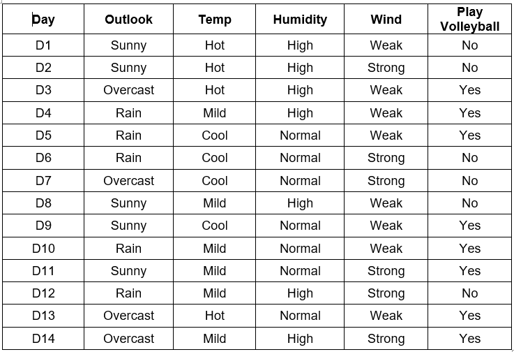
From the above example dataset, we are required to construct a decision tree to help us decide whether we should play volleyball based on the weather conditions.

To construct a decision tree, we need to pick the features that will best guide us to make a viable decision on whether we should play or not play volleyball.

We can't randomly select a feature from the dataset to build the tree, so Entropy and information gain are good criteria for this problem.

To begin with, we have four features we need to consider:

• Outlook
• Temp
• Humidity
• Wind

A decision tree has various parts, the root node, internal nodes, and leaf nodes. Read more on our Decision Tree and Random Forests article.

Finding the root node feature

Since we can not just pick one of the features to start our decision tree, we need to make calculations to get the feature with the highest information gain from which we start splitting.

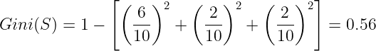
Calculate the entropy of the entire dataset(Entropy(S))

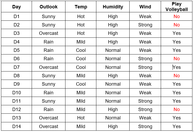
We can see that we have 5 Noes(or negatives) and 9 Yeses(or positives). The total number of entries is 14.

The entropy of the whole dataset is:

import math

S = -(9/14) * math.log2(9/14) - (5/14) * math.log2(5/14)
S
# 0.9402859586706311

Calculate the information gain for the Outlook feature

Outlook has 3 attributes:

• Sunny
• Overcast
• Rain.

So we will calculate the entropy of each of these attributes(Sv) as follows:

We have 5 Sunny attributes for Outlook:

• 3 negative Sunny Outlooks(When Play Volleyball is No).
• 2 positive Sunny Outlooks(When Play Volleyball is Yes).

Let's calculate:

import math

entropy_S_sunny = -(2/5) * math.log2(2/5) - (3/5) * math.log2(3/5)
entropy_S_sunny
# 0.9709505944546686

We have 4 Overcast attributes for Outlook:

• 0 negative Overcast Outlooks.
• 4 positive Overcast Outlooks.

Let's calculate:

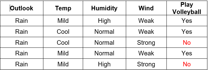
We have 5 Rain attributes for Outlook:

• 2 negative Rain attributes.
• 3 positive Rain attributes.

Let's calculate:

import math

entropy_S_rain = -(3/5) * math.log2(3/5) - (2/5) * math.log2(2/5)
entropy_S_rain
# 0.9709505944546686

The information gain for Outlook

We have the following Entropies:

• Entropy(S) = 0.94
• Entropy(S_Sunny) = 0.97
• Entropy(S_Overcast) = 0
• Entropy(S_Rain) = 0.97

We use the formula for information gain to calculate the gain.

So:

Information gain for Outlook is 0.24.

Similarly, we have to calculate the information gain for the other features.

Calculate the information gain for the Temp feature

Temp has 3 attributes:

• Hot
• Mild
• Cool

Since we already have the entropy for the entire dataset(Entropy(S)), we will calculate the entropy of each attribute(Entropy (Sv)) of Temp, just as we did with Outlook.

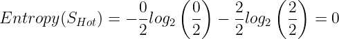
The entropy of Hot:

import math

entropy_S_hot = -(2/4) * math.log2(2/4) - (2/4) * math.log2(2/4)
entropy_S_hot
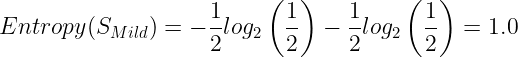
# 1.0

The entropy of Mild:

import math

entropy_S_mild = -(4/6) * math.log2(4/6) - (2/6) * math.log2(2/6)
entropy_S_mild
# 0.9182958340544896

The entropy of Cool:

import math

entropy_S_cool = -(3/4) * math.log2(3/4) - (1/4) * math.log2(1/4)
entropy_S_cool

# 0.8112781244591328

Calculate the information gain for the Temp feature:

Information gain for Temp is 0.03.

Similarly, calculate the information gain for Humidity and Wind. All information gain values will be:

• Gain(S, Outlook) = 0.24
• Gain(S, Temp) = 0.03
• Gain(S, Humidity) =  0.15
• Gain(S, Wind) = 0.04

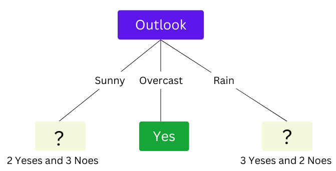
Note, for Sunny and Rain branches, we can not easily conclude a yes or a no since we have events where Play Volleyball is yes and Play volleyball is no. That means that their entropy is more than zero and hence impure. So we need to split them.

Finding the internal nodes

We will calculate information gain for the rest of the features when the Outlook is Sunny and when the Outlook is Rain:

Splitting on the Sunny attribute

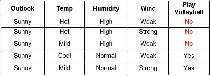
Calculate the information gain for Temp

Values(Temp) = Hot, Mild, Cool.

The entropy for Hot:

The entropy for Mild:

The entropy for Cool:

The Information gain for Temp:

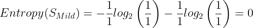
Calculate the information gain for Humidity

Values(Humidity) = High, Normal.

The entropy for Sunny:

Entropy(S_Sunny) = 0.97

The entropy for High:

Entropy(S_High) = 0

Then entropy for Normal:

Entropy(S_Normal) = 0

The Information gain for Humidity:

Calculate the information gain for Wind

Values(Wind) = Strong, Weak.

The entropy for Sunny:

Entropy(S_Sunny) = 0.97

The entropy for Strong:

Entropy(S_Strong) = 1.0

The entropy for Weak:

The Information gain for Wind:

Humidity gives the highest information gain value(0.97). So far, our Tree will look like this:

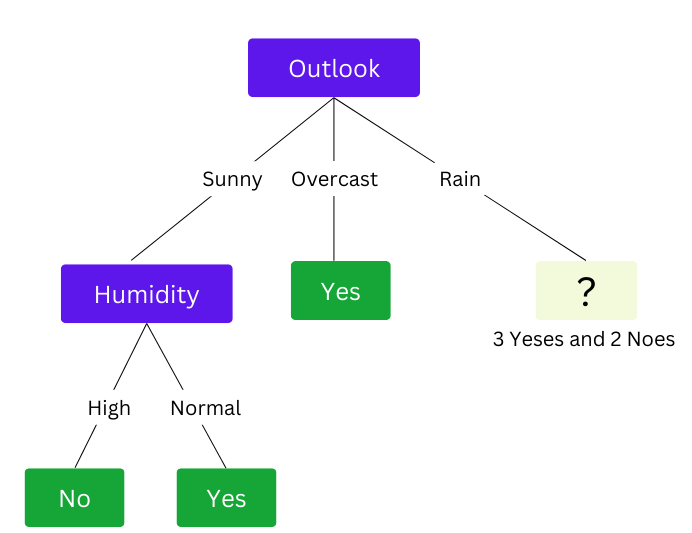
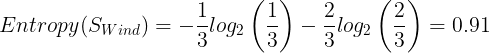
Splitting on the Rain attribute

Calculate the information gain for Temp

Values(Temp) = Mild, Cool

The entropy for Mild:

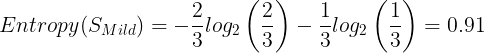
The entropy for Cool:

Entropy(S_Cool) = 1.0

The information gain for Temp:

Calculate the information gain for Humidity

Values(Humidity) = High, Normal.

The entropy for High:

Entropy(S_High) = 1.0

The Entropy for Normal:

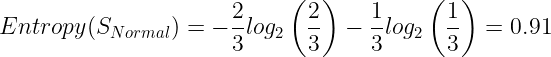
The Information gain for Humidity:

Calculate the information gain for Wind

Values(Wind) = Strong, Weak.

The entropy for Strong:

Entropy(S_Strong) = 0

The entropy for Weak:

Entropy(S_Weak) = 0

The information gain for Wind:

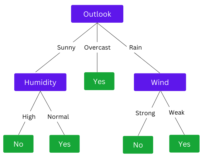
Wind gives the highest information gain value(0.97). Now we can complete our Decision Tree.

A complete decision tree with Entropy and Information gain criteria

Gini impurity

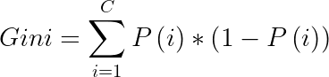
Gini impurity is the probability of incorrectly classifying a random data point in a dataset. It is an impurity metric since it shows how the model differs from a pure division.

Unlike Entropy, Gini impurity has a maximum value of 0.5(very impure classification) and a minimum of 0(pure classification).

Gini impurity has the following formula:

Where:

If we have a dataset of classes C, P(i) is the probability of picking a data point of class i, and 1-P(i) is the probability of not picking a data point of class i.

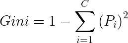
When the above formula is simplified, we get the following formula:

Let's take the following dummy dataset, for example. We will use the Gini criteria to construct a decision tree from it.

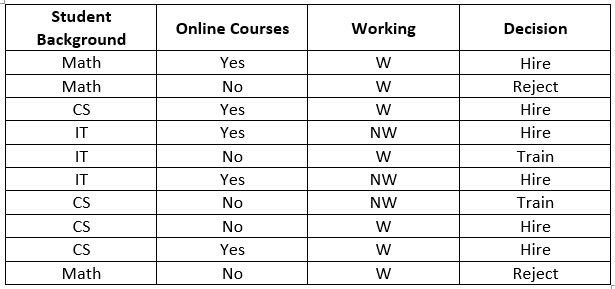
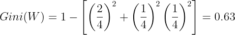
First, we calculate the Gini for the whole dataset. We have 3 possible output variables:

• Hire - 6 instances.
• Reject - 2 instances.
• Train - 2 instances.

So the Gini will be:

Gini for the entire dataset is 0.56.

Next, we calculate the Gini for the features to decide on the root node.

Calculate Gini for Student Background

The "Student Background" feature has 3 possible values:

• Math - 3 instances.
• IT - 3 instances.
• CS - 4 instances.

Gini for when the "Student Background" is in Math. There are 2 examples when the decision is Hire and 1 when the decision is Reject. So:

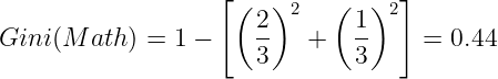
We do the same for IT and CS, where all three Gini values will be:

• Gini(Math) = 0.44.
• Gini(CS) = 0.38.
• Gini(IT) = 0.44.

Now we calculate the weighted average for "Student Background":

w_avrg = 0.44*(3/10) + 0.38*(4/10) + 0.44*(3/10)
w_avrg

# 0.41600000000000004

Gini for the Student background feature is 0.416.

Calculate Gini for Online Courses

The "Online Courses" feature has two possible values:

• Yes - 5 instances.
• No - 5 instances.

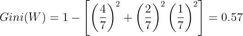
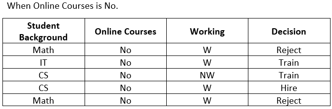
Gini for when the "Online Courses" is No. There is 1 example when the "Decision" is Hire, 2 examples when the "Decision" is Reject, and 2 examples when the "Decision" is "Train". So:

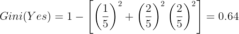
The Gini for when the "Online Courses" is Yes is 0 since there are 5 out of 5 instances when the decision is Hire.

Now we calculate the weighted average for "Online Courses":

w_avrg = 0*(5/10) + 0.64*(5/10)
w_avrg

# 0.32

Gini for the Online Courses feature is 0.32.

Calculate Gini for Working

The "Working" feature has 2 possible values:

• W(Working) - 7 instances.
• NW(Not working) - 3 instances.

Gini for when the "Working" is W. There are 4 examples when the "Decision" is Hire, 2 examples when the "Decision" is Reject, and 1 example when the "Decision" is Train. So:

We do the same for Not Working, and the Gini values will be :

• Gini(W) = 0.57.
• Gini(NW) = 0.44.

Calculate the weighted average for "Woking":

w_avrg = 0.57*(7/10) + 0.44*(3/10)
w_avrg

# 0.5309999999999999

Gini for the Working status feature is 0.53.

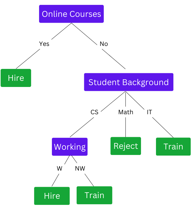
To decide on the root node, we check the Gini values achieved by each feature. The lower the Gini value, the better.

• Gini(Student Background) = 0.416
• Gini(Online Courses) = 0.32.
• Gini(Working Status) = 0.53.

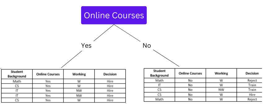
Since the classification when "Online Course" is Yes results in one decision, we get a leaf node as Hire.

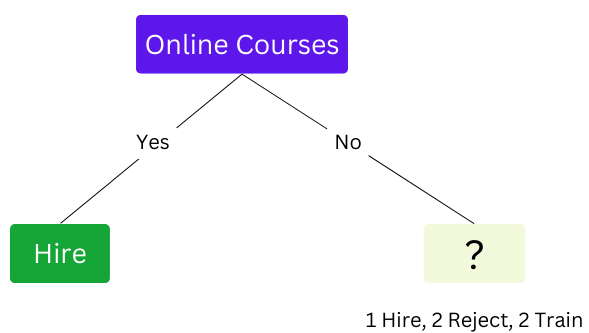
Since the right node is not pure, we will further split it.

We will compute the Gini for when:

• "Online Courses" is No, and "Student Background"
• "Online Courses" is No and "Working."

Calculate the Gini for "Student Background"

When "Online Course" is No, and "Student Background" is Math, we have 2 instances with similar Decision(Reject). So the Gini value will automatically be 0.

When "Online Course" is No, and "Student Background" is IT, we have 1 instance: "Decision" is Train. So the Gini value will be 0.

When "Online Course" is No, and "Student Background" is CS, we have 2 instances: "Decision" is Train. So the Gini value will be 0.5.

Weighted average:

w_avrg = 0*(2/5) + 0*(1/5) + 0.5*(2/5)
w_avrg
# 0.2

Gini For "Student Background" is 0.2.

Calculate the Gini for "Working"

When Online Course is No, and "Working" is W. We get the Gini as:

When "Online Course" is No, and "Working" is NW, we have 1 instance so the Gini value is 0:

Weighted average:

w_avrg = 0.63*(4/5) + 0*(1/5)
w_avrg
# 0.5

Gini For "Working" is 0.5.

Since "Student Background" has the least Gini value, it will be the next internal node. So now we can complete the decision tree.

A complete decision tree with Gini criteria

Final thoughts

In this article, we have learned three splitting criteria used by decision trees. In general practice, we don't do all these calculations manually. When building the decision tree model, an algorithm will do all these calculations in the back end.

Check out our article on decision trees and random forests to learn how to build and optimize them.

The Complete Data Science and Machine Learning Bootcamp on Udemy is a great next step if you want to keep exploring the data science and machine learning field.

Follow us on LinkedIn, Twitter, and GitHub, and subscribe to our blog, so you don't miss a new issue.