NumPy tutorial(Everything you need to know about NumPy with examples)

So, you have decided to venture into data science and machine learning, and maybe you have been using Python for other projects or you are new to Python. Well, you just pointed yourself to the right path. However, to venture into data science and machine learning, you will need to know the libraries used in the field.

This document will get you up to speed with one of the most fundamental Python libraries you need to know— NumPy.

New to Python? We advise that you first visit our Python for data science tutorial before starting on NumPy.

What is NumPy

NumPy, shortened form for Numerical Python, is a powerful library for working with arrays. It has a multidimensional array object and various utilities for working with these arrays.NumPy forms a base for other Python libraries like Pandas, Matplotlib, Scikit-learn, and Scipy.

NumPy is an alternative to Python lists because it overcomes slower executions by using the multidimensional array object to perform complex logical and mathematical operations. This means that it is faster than Python lists in performing complex operations.

Getting started with NumPy

The quickest way to use NumPy is to download and install the Anaconda Distribution. The Anaconda distribution of Python ships with NumPy and various data science packages.

Follow these instructions to install Anaconda in your respective operating system.

Installation — Anaconda documentation

Docs Home Anaconda Home More Help & Support 2022 Anaconda, Inc. All Rights Reserved. Privacy Policy

If you have Python and pip installed, run pip install numpy from your terminal or cmd.

pip install numpy

To start using NumPy in whichever environment you are, you need to import it.

Now we are ready to do magic!

NumPy arrays

The NumPy ndarray is an N-dimensional array object that stores a group of similar types of data. By default, each element in the ndarray is an object of data type object(dtype).

Creating ndarray object in NumPy

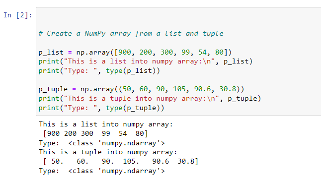
We create a NumPy array with the array() function. When a Python list or tuple is passed into the array function, it is automatically converted to a ndarray. It is accessed with zero-based indexing, like in regular arrays.

The array() function accepts a couple of parameters:

1. object specifies the object, which can be a list, tuple, dictionary, etc.
2. dtype is mostly used when we are type casting; thus, it is optional. It specifies the data type passed to the array. NumPy will automatically determine the appropriate type required to hold the array object if we do not define it. dtype also checks the data type.
3. order  specifies the memory layout of the array. The orders are 'K', 'C', 'F', 'A'.
4. copy  when set to true, the object is copied.
5. ndmin specifies the number of dimensions we want our resulting array to have. ndmin is also used to check the dimensions of our array.
6. subok when set to true, subclasses will pass through. Otherwise, the resulting array is forced to be a base class array(default).

Converting a Python list and tuple to a NumPy array object

Passing a Python list or tuple to numpy.array  converts them to NumPy arrays. You can confirm that they have become NumPy arrays using type().

Dimensions in NumPy arrays

Zero-dimensional arrays (0-D) are values in the array.

One-dimensional arrays (1-D) are the basic array dimensions. They contain the 0-D arrays as their elements.

Two-dimensional arrays(2-D) are arrays with 1-D arrays as their elements.

Three-dimensional arrays(3-D) are arrays with 2-D arrays, also called matrices.

An array can have multiple dimensions. To specify the number of dimensions we want in our array, we use the ndim parameter.

NumPy array creation functions

One way to create NumPy arrays is by converting Python lists and tuples using np.array as we have done above. There are other essential functions defined in NumPy that we can use to create the arrays. Let's mention some of them.

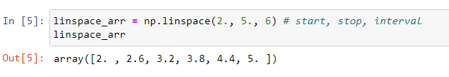
np.linspace needs at least three inputs. start,end,step. It creates a 1-D array with a specified number of values spaced equally between the beginning and end values. step specifies the space between values.

np.arange expects at least three inputs. start,end, step. It creates a 1-D array that has incrementing values. Its advantage over Python's range() function is that it allows the generation of a series of values that are not integers. range() gives an error if you try to do that.

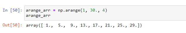
If you only provide one argument to the arange() function, it will work with: start = 0 stop = 'argumentpassed' step = 1.

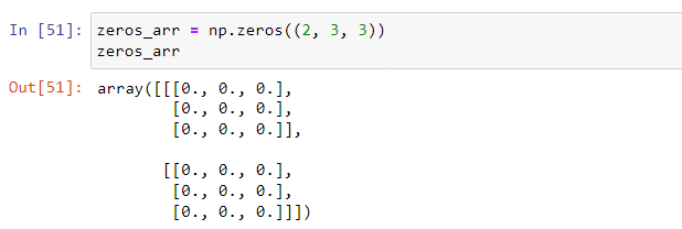
np.zeros creates an array filled with zeros and with the specified shape.

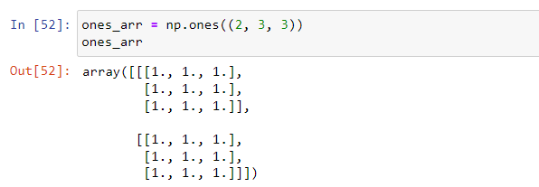
np.ones is similar to np.zeros but creates an array with ones.

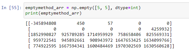
np.empty creates an array with the given shape and dtype without having to initialize the array.

NumPy data types

NumPy has a variety of scalar data types. Each of its built-in data types has a character code that identifies it. The character code are:

• i – character code is for integers(int8, int16, int32, int64, intp).
• u – character code for unsigned integers(uint8, uint16, uint32, uint64).
• f – character code for floats(float16, float32, float32).
• c – character code for complex floats(complex64, complex128).
• S – character code for string.
• O – character code for object.
• M – character code for datetime.
• b – character code for boolean.
• U – character code for unicode string.

The NumPy dtype

As we mentioned above, items of the NumPy array are NumPy dtypes , where each data type object has a fixed memory block relative to the array.

We create the dtype object with the numpy.dtype() constructor. This constructor takes in three parameters which are:

• Object representing the object that we want to be converted to dtype.
• Align can be set to either True or False. If set to true, it will add padding to make the object equal to a C-struct.
• Copy generates a copy of the dtype object.

For example, let's create simple data types containing various scalar data types defined in NumPy. This can be done in two ways:

1. Using the data type names

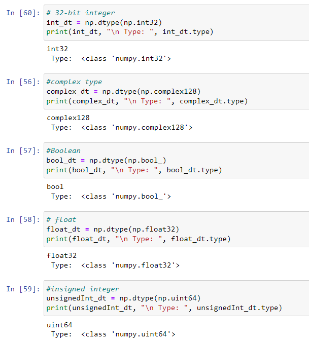
Notice that the data types we have created are exactly of data type NumPy object.

2. Using the character codes

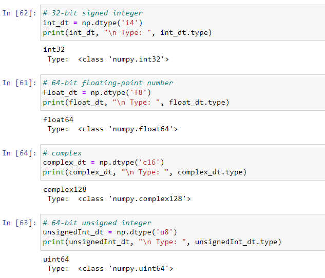
To check the data type of an object, we use dtype like:

Creating structured data types

A structured data type is a collection of fields where each field has a name, a data type, and a byte offset. The data type field can be any NumPy datatype while NumPy automatically determines the byte offset, but you can specify it.

Here's how to create the structured data types.

Creating a list of tuples where each field has one tuple

Every tuple will have the format (fieldname, datatype, shape). Shape here is optional and contains a tuple of integers defining the shape.

If you leave the fieldname empty, it will automatically be assigned a default name of the form f# where the # is the index of the field counting from index 0.

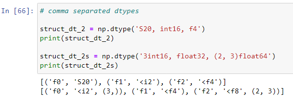
Creating a list of comma-separated dtype specifications

Here, the fieldnames and the byte offset are assigned automatically. The field names are given names  f0, f1, f2... according to the index of the field. Notice in the second example that we can specify the shape before the data type.

Creating a dictionary of field parameter arrays

Remember Python dictionaries? They store data in key value pairs. Now when we create the structured dtype with them, we will have at-least four keys to use, which are:

• names  should have a list of field names [].
• formats must be a list of dtypes of the same length.
• offsets optional. The value should have a list of integer byte offsets.
• itemsize optional. The value must be an integer describing the total size of the dtype.

Structured arrays

These are arrays whose dtype is a structured data type.

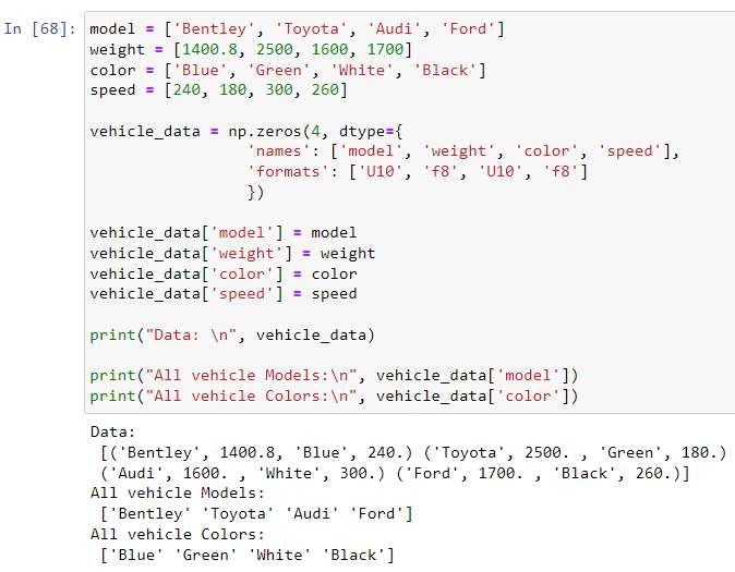
Suppose we had different categories of data about some car models; for example model, weight, color and speed and we want to store this information for use in a Python program.

We can store these data in lists like this:

However, we cannot deduce how the arrays are related from the above data. To represent them more neatly, we could store the data in NumPy structured arrays.

Indexing NumPy arrays

Indexing NumPy array is accessing an array element by referencing it with the syntax x[obj] where x represents the array and obj the reference to the element. We can use indexing methods to access these elements in the array.

Indexing a single element

We use the 0-based indexing to index a single element. We can access an element in a 1-D array, 2-D array, or 3-D array. We can also do negative indexing.

Let's look at how we can do indexing for the various dimensions.

Slicing

When we slice an array, we extract its elements from a certain index to a specified index. We use the x[obj] syntax only that this time the obj will be a slice object, an integer, or a tuple of both.

We pass in three arguments in the [obj] construct:

• start specifies the index we want to start extracting from. When we don't specify it, it is assumed to be 0.
• end determines the end index where the slicing will stop. If not specified, the length of the array is used. This stop index is not included in the results.
• step  dictates the interval for picking the elements. It is 1 by default.

The entire syntax for slicing would look like this: x[start:end:step] .

NumPy array shapes and reshaping

An array's shape is the number of elements in each dimension. To know the shape of an array, we use the shape attribute, which returns a tuple.

From the code we see that:

• the 1-D array shape is (5,) which means that the array is 1 dimension and has 5 elements.
• the 2-D array shape is (2, 4)  indicating that it is a 2-dimensional array where the first dimension has 2 elements(rows) and the second dimension has 4(columns).
• the 3-D array shape is (2, 2, 2) which means that it is a 3-dimensional array where each dimension has 2 rows and 2 columns.

Reshaping NumPy arrays

Reshaping means changing the shape of the array in use. We can reshape an array to any dimension we want.

Broadcasting Numpy arrays

Sometimes when we perform mathematical operations in real-world problems, we mustn't be constrained by the fact that operations on two arrays must be the same shape for the operation to work.

For example:

Adding two arrays with different shapes returns an error from the code above. This is where broadcasting comes to play.

Broadcasting is the ability of NumPy to work with different shapes and enable us to perform operations as we require. However, it is only possible under the satisfaction of the following rules:

1. If the two arrays differ in their dimensions, the shape of the array with a smaller ndim is prepended with one (1) on its left side.
2. If the shape of the two arrays does not match in any dimension, then the array with the shape of 1 in that dimension is stretched to match the other shape.
3. If in any dimension the sizes defer and none is equal to 1, the operation fails.

Other rules are:

• The two arrays have the same shape.
• The two arrays have the same number of dimensions and the length of each ndim is equal or 1.

From the example above, the sum of array_a and array_b is successful despite their shapes being different, thanks to the rules.

Let's see how:

1. Since the dimensions of both arrays are different, the first broadcasting rule is invoked.
2. The shape of array_b which is the smaller one is prepended with ones. From (3,) to (1, 3) which now matches array_a (4, 3).
3. Since now the shapes are equal, the dimensions are compiled from the trailing end. Since the length of dimension at the trailing end in both (...,3) and (...,3) is true, the compilation is moved to the next dimension in both (4, ) and (1, ). Since the sizes of the dimensions are different, NumPy checks whether any of them is 1, and since one of them is 1, the operation is done by invoking the second rule where the array_b is stretched to match the other shape.

4. The resultant array is of the shape (4, 3). The resulting shape is always equal to the shape of the higher array.

Let's see an example of a failed broadcast.

We can evaluate why this failed.

1. Both arrays' shapes are different, so the first rule is invoked.
2. The shape of the smaller array array_b is prepended with 1. It takes the shape  (1, 4) from (4,). Matches the shape (4, 3) of array_b.
3. NumPy now compiles the dimensions of each array from the trailing end. Since the length of dimension at the trailing end in both (...,3) and (...,4) is false, NumPy checks if one of the dimensions here is 1. Since the dimensions from the trailing end are not equal and none of them is 1, NumPy automatically returns that both arrays can not be broadcasted as the requirements are not met.

The second dimensions from the trailing end are not evaluated if the first rule is not met.

NumPy axis directions

Iteration in NumPy happens through a type of axis called the NumPy axis. Each operation has a specific iteration process to get to a particular result. There are two iteration processes the Column order('C') for the column axis and Fortran Order('F') for the row axis.

• Axis 0 runs vertically through rows of the multidimensional array and performs column-wise operations.
• Axis 1 runs horizontally across the multidimensional array's column and performs row-wise operations.

Iterating over NumPy arrays

Iterating over an array means going through each element one by one. We can use Python's for loop to do so as we deal with multidimensional arrays in NumPy.

We can get values from 1-D, 2-D, and 3-D arrays.

Using for loops to iterate over these arrays is pretty simple. However, let's say we are working with an array with higher dimensionalities, maybe 6-D and higher. We would have to nest many for loops to get the values.

NumPy has a multidimensional iterator object called nditer() that addresses this problem.

Modifying array elements

We can modify elements in the array while iterating. Some parameters used in nditer object include:

• flags a sequence of str: optional, for example, (flags = ['external_loop', 'buffered']).
• op_flags  a list of str: optional, for example,(op_flags = ['readwrite' or 'writeonly']).
• op_dtypes a dtype or tuple of dtypes for example, (op_dtypes = ['S'])
• order – {‘C’, ‘F’, ‘A’, ‘K’}: optional, for example, (order = 'C')

Let's take a look at an example involving multiplying each element with 3 while iterating.

Here's another example showing how to change the dtype of the elements while iterating.

Notice that we need extra space to change the dtype since NumPy doesn't alter the dtype of where the element is in the array. So we specify a buffer value in the flags parameter.

Numpy string functions

NumPy has a couple of functions to enable us to work on arrays of type string.

np.char.add() concatenates elements in two arrays.

np.char.multiply() returns a string with multiple concatenations.

np.char.center() returns a copy of the string. The original string is centered and padded on both sides with fillchar.

np.char.lower() converts the array elements to lowercase and returns the string.

np.char.upper() returns an array with elements converted to uppercase.

np.char.capitalize() returns a copy of the string with its first letter in uppercase.

np.char.join() returns a string with each of its characters joined by a separator.

np.char.split() returns a list of words separated by the specified separator or by default white space.

At this point, you have learned basic array operations like:

• Finding the data type of an array usingdtype.
• Checking the dimension of an array using ndim.
• Finding the size of each element in the array using itemsize.
• Viewing the size of an array withsize.
• Finding the shape of an array using shape.
• Reshaping an array withreshape().
• Slicing an array using x[start:end:step].

In the following section, we will introduce more operations you can perform on NumPy arrays.

NumPy mathematical operations

Let's look at some of the mathematical operations you can perform with Numpy.

Rounding

Rounding array elements to the desired precision can be done with various functions.

• np.around() evenly rounds to a certain number of decimals. It rounds to the nearest even number exactly halfway between rounded decimal values.
• np.floor() returns the floor(largest integer) of the array element.
• np.ceil() gives the ceiling(smallest integer) of the array element.
• np.trunc() returns a truncated value(fractional part discarded) of the array element.
• np.fix() rounds array element towards zero.

Trigonometry

NumPy also ships with some trigonometry functions:

• np.sin returns the trigonometric sine of each element.
• np.cos computes the cosine of each element.
• np.tan calculates the tangent of each element.
• np.arcsin returns the inverse of sine.
• np.arccos to calculate the inverse of cosine.
• np.arctan for computing the inverse of the tangent.

Finding extremes in NumPy array

The following functions are used to compute extremes in NumPy:

• np.amax() returns the maximum of an array or maximum along an axis.
• np.amin() returns the minimum of an array or minimum along an axis.
• np.argmax() returns the indices of the maximum value along the axis

NumPy arithmetic operations

We can perform arithmetic operations on NumPy arrays. These operations include adding, subtracting, multiplication and division.

When working with these operations, we must ensure that the arrays have adhered to the broadcasting rules we have learned or have the same shape. Otherwise, these operations will not work.

Here are some common NumPy math functions:

• np.add() adds two arrays.
• np.sum() returns the total sum of array elements.
• np.subtract() subtract two arrays.
• np.divide() divides two arrays.
• np.multiply() multiplies two arrays.
• np.reciprocal() returns reciprocal argument of the element. Values with absolute values of more than one return 0.
• np.mod() returns the modulus of corresponding elements
• np.power() returns the first array raised to the power of corresponding elements in the second array.

NumPy statistical operations

You can also use NumPy to perform statistical computations. Let's look at some of the supported statistical functions.

Square root

NumPy's np.sqtr()  returns a non-negative square root of each element in the array.

Mean

Mean finds the sum of all the array elements and then divides the sum by the number of elements in the array. We can also specify the axis for the operations.

We find the mean using the np.mean() function.

Median

The Median is the middle element in the array. NumPy can find the median for both 1-D and multidimensional arrays.

We compute the median using the np.median() function.

Variance

Variance is the average of square deviations.

We calculate the variance using the np.var() function.

Standard deviation

Standard deviation is the square root of the average square deviations(variance).

Standard deviation is computed using the np.std() function.

Generating random numbers

When we generate random numbers, we create numbers we can not logically predict at any given moment.

NumPy has a random module that we need to import to work with random numbers. Here's what we can do with this module:

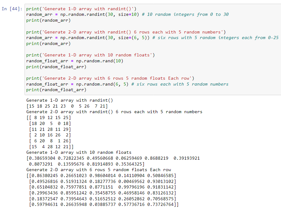
Generate random integers numbers and floats:

Generate random arrays:

We can generate random numbers from an array with the choice() method. The method takes an array of values and randomly returns one of them. We can also specify size in the method to generate an array of the specified shape.

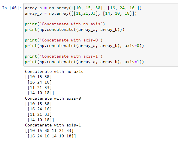
Concatenating arrays

NumPy's np.concatenate() is used to join two or more arrays of the same shape.

It is essential to note this function does not behave like in database join. What it does is stack the arrays either vertically or horizontally.

We can also specify the axis on which we want to join the arrays.

Sorting NumPy arrays

While working with arrays, sometimes we require a sorted array for computation. NumPy has numpy.sort() function for this purpose. The code example below clearly shows how we can sort arrays.

Filtering NumPy arrays

Filtering arrays means taking elements from an existing array and making another array out of these values.

We use a boolean index list consisting of True and False values where when a value at a certain index is True, that value is included in the resultant array; otherwise, if the value at a certain index is False, it is excluded.

Searching values in arrays

We can search a value from an array. NumPy provides a method  called where() which returns the index of the value in the array based on a condition.

Final thoughts

This article covers a significant chunk of what you need to understand to start using NumPy in your data science and machine learning journey. Specifically, we have learned:

• What is NumPy?
• How to create NumPy arrays.
• Data types in NumPy.
• Creating structured data types in NumPy.
• Built-in NumPy functions.
• Indexing NumPy arrays.
• NumPy string functions.
• Filtering values in NumPy arrays.
• Operations on NumPy arrays.
• Searching values in NumPy arrays.

...just to mention a few.

The Complete Data Science and Machine Learning Bootcamp on Udemy is a great next step if you want to keep exploring the data science and machine learning field.

Follow us on LinkedIn, Twitter, GitHub, and subscribe to our blog, so you don't miss a new issue.