
Create U-Net from scratch (Image segmentation with U-Net with Keras and TensorFlow)

In the Implementing Fully Convolutional Networks (FCNs) from scratch in Keras and TensorFlow article, you saw how to build an image segmentation model with FCNs. However, due to the model's limitations, it did not perform very well in the segmenting task. In this post, you will see how to improve segmenting using a different model known as U-Net.
How does the U-Net model work?
The U-Net architecture was proposed in the U-Net: Convolutional Networks for Biomedical Image Segmentation paper in 2015. U-Net is an extension of Fully Convolutional Neural Networks; it, therefore, doesn't have any fully connected layers.
In a nutshell, U-Net works as follows:
- It uses a contracting path to downsample the image features.
- Upsamples the features using an expansive path.
- Concatenates features from the downsampling process during upsampling.
The contracting and expansive paths mirror each other. The name U-Net comes from the shape of the network, which forms a U-shape.
mlnuggets newsletter
Join the newsletter to receive these technical dives in your inbox.
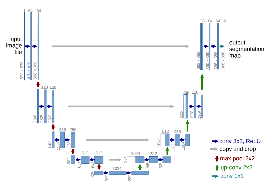
High-resolution features from the contracting path are combined with the upsampled output to improve the network's localization capacity.
Processing data for image segmentation
Let's now look at how to build a U-Net model using the 2018 Data Science Bowl dataset from Kaggle. Participants in this competition were tasked with creating a network to identify nuclei from various images. You can follow along using this notebook.
The training data contains images and their corresponding masks. Each image can have multiple masks.
Let's start by extracting and resizing the training and testing set. Since the U-Net model has no fully connected layers, it can accept images of arbitrary size, but you still want to resize them to reduce the computation time.
import tensorflow as tf
import os
import random
import numpy as np
from tqdm import tqdm
from skimage.io import imread, imshow
from skimage.transform import resize
import matplotlib.pyplot as plt
from sklearn.model_selection import train_test_split
from zipfile import ZipFile
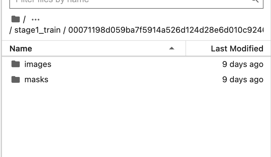
with ZipFile("../input/data-science-bowl-2018/stage1_train.zip","r") as zip_ref:
zip_ref.extractall("./stage1_train")
with ZipFile("../input/data-science-bowl-2018/stage1_test.zip","r") as zip_ref:
zip_ref.extractall("./stage1_test")
seed = 42
np.random.seed = seed
IMG_WIDTH = 128
IMG_HEIGHT = 128
IMG_CHANNELS = 3
TRAIN_PATH = 'stage1_train/'
TEST_PATH = 'stage1_test/'
train_ids = next(os.walk(TRAIN_PATH))[1]
test_ids = next(os.walk(TEST_PATH))[1]
X = np.zeros((len(train_ids), IMG_HEIGHT, IMG_WIDTH, IMG_CHANNELS), dtype=np.uint8)
y = np.zeros((len(train_ids), IMG_HEIGHT, IMG_WIDTH, 1), dtype=bool)
__author__ = "Sreenivas Bhattiprolu"
__license__ = "Feel free to copy, I appreciate if you acknowledge Python for Microscopists"
# Credits https://github.com/bnsreenu/python_for_microscopists
"""
@author: Sreenivas Bhattiprolu
"""
print('Resizing training images and masks')
for n, id_ in tqdm(enumerate(train_ids), total=len(train_ids)):
path = TRAIN_PATH + id_
img = imread(path + '/images/' + id_ + '.png')[:,:,:IMG_CHANNELS]
img = resize(img, (IMG_HEIGHT, IMG_WIDTH), mode='constant', preserve_range=True)
X[n] = img #Fill empty X_train with values from img
mask = np.zeros((IMG_HEIGHT, IMG_WIDTH, 1), dtype=bool)
for mask_file in next(os.walk(path + '/masks/'))[2]:
mask_ = imread(path + '/masks/' + mask_file)
mask_ = np.expand_dims(resize(mask_, (IMG_HEIGHT, IMG_WIDTH), mode='constant',
preserve_range=True), axis=-1)
mask = np.maximum(mask, mask_)
y[n] = mask
# test images
test_images = np.zeros((len(test_ids), IMG_HEIGHT, IMG_WIDTH, IMG_CHANNELS), dtype=np.uint8)
sizes_test = []
print('Resizing test images')
for n, id_ in tqdm(enumerate(test_ids), total=len(test_ids)):
path = TEST_PATH + id_
img = imread(path + '/images/' + id_ + '.png')[:,:,:IMG_CHANNELS]
sizes_test.append([img.shape[0], img.shape[1]])
img = resize(img, (IMG_HEIGHT, IMG_WIDTH), mode='constant', preserve_range=True)
test_images[n] = img
print('Done!')Next, split the data into a training and testing set.
X_train, X_test, y_train, y_test = train_test_split(X, y, test_size=0.33, random_state=42)You can visualize a sample image and the corresponding mask using Matplotlib.
image_x = random.randint(0, len(X_train))
plt.axis("off")
imshow(X_train[image_x])
plt.show()
plt.axis("off")
imshow(np.squeeze(y_train[image_x]))
plt.show()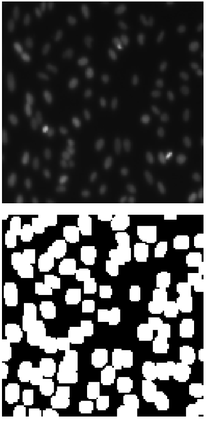
Define U-Net model for image segmentation
In this article, let's create a U-Net model that differs slightly from the original paper implementation.
The contracting path will have five blocks with the following layers :
- Convolution
- Drop out
- Batch normalization
- ReLu
- Max pooling
The expansive path will be asymmetric with the contracting having these layers:
- Upsampling – Conv2DTranspose
- Concatenate to combine upsampled and downsampled features
- Batch normalization
- ReLU
The final output is obtained by a Conv2D layer with a sigmoid activation and a stride of 1.
num_classes = 1

inputs = tf.keras.layers.Input((IMG_HEIGHT, IMG_WIDTH, IMG_CHANNELS))

#Contraction path
c1 = tf.keras.layers.Conv2D(16, (3, 3), activation='relu', kernel_initializer='he_normal', padding='same')(inputs)
c1 = tf.keras.layers.Dropout(0.1)(c1)
c1 = tf.keras.layers.Conv2D(16, (3, 3), activation='relu', kernel_initializer='he_normal', padding='same')(c1)
b1 = tf.keras.layers.BatchNormalization()(c1)
r1 = tf.keras.layers.ReLU()(b1)
p1 = tf.keras.layers.MaxPooling2D((2, 2))(r1)

c2 = tf.keras.layers.Conv2D(32, (3, 3), activation='relu', kernel_initializer='he_normal', padding='same')(p1)
c2 = tf.keras.layers.Dropout(0.1)(c2)
c2 = tf.keras.layers.Conv2D(32, (3, 3), activation='relu', kernel_initializer='he_normal', padding='same')(c2)
b2 = tf.keras.layers.BatchNormalization()(c2)
r2 = tf.keras.layers.ReLU()(b2)
p2 = tf.keras.layers.MaxPooling2D((2, 2))(r2)

c3 = tf.keras.layers.Conv2D(64, (3, 3), activation='relu', kernel_initializer='he_normal', padding='same')(p2)
c3 = tf.keras.layers.Dropout(0.2)(c3)
c3 = tf.keras.layers.Conv2D(64, (3, 3), activation='relu', kernel_initializer='he_normal', padding='same')(c3)
b3 = tf.keras.layers.BatchNormalization()(c3)
r3 = tf.keras.layers.ReLU()(b3)
p3 = tf.keras.layers.MaxPooling2D((2, 2))(r3)

c4 = tf.keras.layers.Conv2D(128, (3, 3), activation='relu', kernel_initializer='he_normal', padding='same')(p3)
c4 = tf.keras.layers.Dropout(0.2)(c4)
c4 = tf.keras.layers.Conv2D(128, (3, 3), activation='relu', kernel_initializer='he_normal', padding='same')(c4)
b4 = tf.keras.layers.BatchNormalization()(c4)
r4 = tf.keras.layers.ReLU()(b4)
p4 = tf.keras.layers.MaxPooling2D(pool_size=(2, 2))(r4)

c5 = tf.keras.layers.Conv2D(256, (3, 3), activation='relu', kernel_initializer='he_normal', padding='same')(p4)
b5 = tf.keras.layers.BatchNormalization()(c5)
r5 = tf.keras.layers.ReLU()(b5)
c5 = tf.keras.layers.Dropout(0.3)(r5)
c5 = tf.keras.layers.Conv2D(256, (3, 3), activation='relu', kernel_initializer='he_normal', padding='same')(c5)

#Expansive path
u6 = tf.keras.layers.Conv2DTranspose(128, (2, 2), strides=(2, 2), padding='same')(c5)
u6 = tf.keras.layers.concatenate([u6, c4])
u6 = tf.keras.layers.BatchNormalization()(u6)
u6 = tf.keras.layers.ReLU()(u6)


u7 = tf.keras.layers.Conv2DTranspose(64, (2, 2), strides=(2, 2), padding='same')(u6)
u7 = tf.keras.layers.concatenate([u7, c3])
u7 = tf.keras.layers.BatchNormalization()(u7)
u7 = tf.keras.layers.ReLU()(u7)


u8 = tf.keras.layers.Conv2DTranspose(32, (2, 2), strides=(2, 2), padding='same')(u7)
u8 = tf.keras.layers.concatenate([u8, c2])
u8 = tf.keras.layers.BatchNormalization()(u8)
u8 = tf.keras.layers.ReLU()(u8)

u9 = tf.keras.layers.Conv2DTranspose(16, (2, 2), strides=(2, 2), padding='same')(u8)
u9 = tf.keras.layers.concatenate([u9, c1], axis=3)
u9 = tf.keras.layers.BatchNormalization()(u9)
u9 = tf.keras.layers.ReLU()(u9)


outputs = tf.keras.layers.Conv2D(num_classes, (1, 1), activation='sigmoid')(u9)
With the building blocks in place, you can now define the model using the Keras Functional API.
model = tf.keras.Model(inputs=[inputs], outputs=[outputs])
model.compile(optimizer='adam', loss='binary_crossentropy', metrics=['accuracy'])
You can plot the model to see how it looks. As you can see below, it's u-shaped.
tf.keras.utils.plot_model(model, "model.png")
Train U-Net model with Keras and TensorFlow
The next step is to train the model by passing the training and validation data to the Keras fit method. You can also define some callbacks to track the training process, such as the TensorBoard callback.
callbacks = [
        tf.keras.callbacks.EarlyStopping(patience=2, monitor='val_loss'),
        tf.keras.callbacks.TensorBoard(log_dir='logs')]

model.fit(X_train, y_train, validation_data=(X_test,y_test), batch_size=16, epochs=25, callbacks=callbacks)
U-Net model evaluation
With the model trained, you can use the training metrics to plot the training and validation loss.
loss = model.history.history['loss']
val_loss = model.history.history['val_loss']

plt.figure()
plt.plot( loss, 'r', label='Training loss')
plt.plot( val_loss, 'bo', label='Validation loss')
plt.title('Training and Validation Loss')
plt.xlabel('Epoch')
plt.ylabel('Loss Value')
plt.ylim([0, 1])
plt.legend()
plt.show()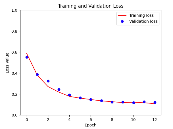
Making predictions using U-Net model
Let's now check the performance of the model on the test set.
def display(display_list):
  plt.figure(figsize=(15, 15))

  title = ['Input image', 'True mask', 'Predicted mask']

  for i in range(len(display_list)):
    plt.subplot(1, len(display_list), i+1)
    plt.title(title[i])
    plt.imshow(tf.keras.utils.array_to_img(display_list[i]))
    plt.axis('off')
  plt.show()

i = random.randint(0, len(X_test))
sample_image = X_test[i]
sample_mask = y_test[i]
prediction = model.predict(sample_image[tf.newaxis, ...])[0]
predicted_mask = (prediction > 0.5).astype(np.uint8)
display([sample_image, sample_mask,predicted_mask])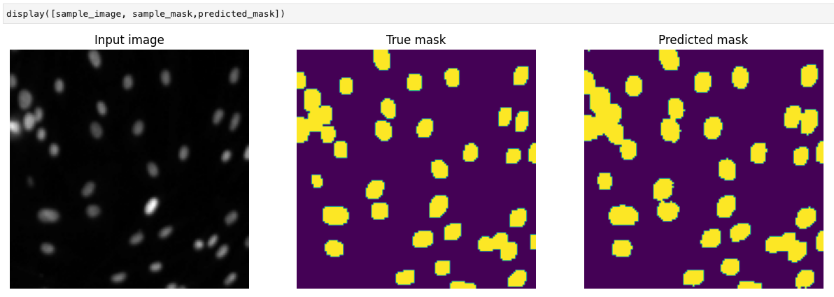
Final thoughts
As you can see from the above image, the segmentation is much better than the one obtained using the Fully Convolutional Network. Therefore, we can conclude that concatenating upsampled and downsampled features help improve the model's segmentation ability.
Whenever you are ready, there are two ways I can help you:
Check out my data science and machine learning courses.
Pick up one of my free or paid data science and machine learning ebooks.