Implementing Fully Convolutional Networks (FCNs) from scratch in Keras and TensorFlow (Build image segmentation model from scratch)

In 2014, Jonathan Long, Evan Shelhamer, and Trevor Darrell proposed solving image segmentation problems using Fully Convolutional Neural Networks(FCNs). FCNs have no fully connected layers.

Image segmentation involves making a prediction for each pixel in an image. FCNs can accept images of any size because they don't have fully connected layers.

This article will explore how to use FCNs to build a model in TensorFlow that can segment nuclei in images. The article assumes that you are familiar with how Convolutional Networks work.  

What are Fully Convolutional Networks (FCNs)?

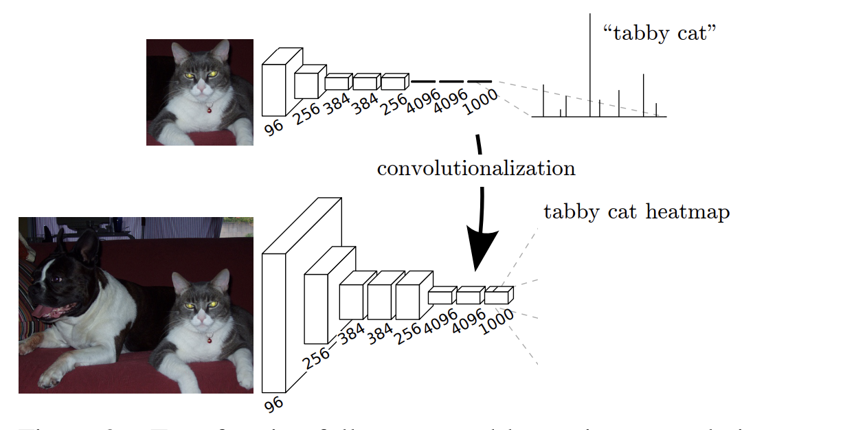
Fully Convolutional Networks (FCNs) are artificial neural networks with no dense layers, hence the name fully convolutional. A Fully Convolutional Network (FCN) is achieved by converting classification networks to convolutional ones.

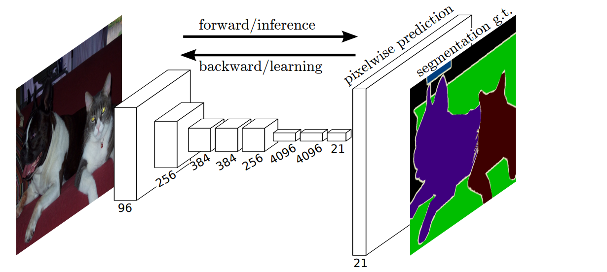
The final output is obtained by converting the dense layers to a convolutional layer with a kernel size of 1 by 1.

The convolutional network will produce coarse output maps. To perform pixel-wise prediction, these coarse outputs need to be upsampled. Upsampling can be thought of as the opposite of convolution – deconvolution. Convolutional operations create features from the image which are smaller than the original image due to the pooling operation. To make pixel-wise predictions, you must go back to the original image.

To obtain the original image, you have to upsample the convolved features. This is done by applying upsampling layers. For example, you might get a 8 by 8 feature map after doing convolution on a 128 by 128 image. You can upsample this feature by a factor of 16 to immediately return to the original image size. However, as you can see below, that will lead to a lot of information being lost, leading to poor segmentation.  

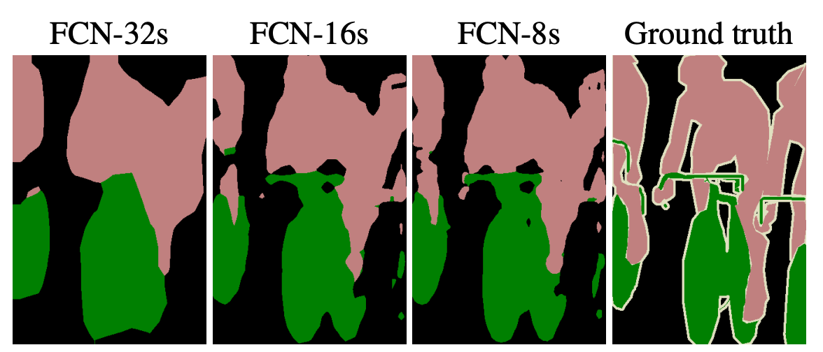
To improve the segmentation detail, you can upsample the 8 by 8 convolved feature map by a stride of two:

• From 8 by 8 to 16 by 16.
• From 16 by 16 to 32 by 32.
• From 32 by 32 to 64 by 64.
• From 64 by 64 to 128 by 128.

This step-by-step upsampling enables the network to recover as many details as possible.  The segmentation can further be improved by adding the upsampling from earlier layers to current ones. You will see this in the Keras implementation.  

Implement FCNs to find the nuclei in divergent images

Let's now look at how to build a Fully Convolutional Neural Network using the 2018 Data Science Bowl dataset from Kaggle. Participants in this competition were tasked with creating a network to identify nuclei from various images.

Prepare training data

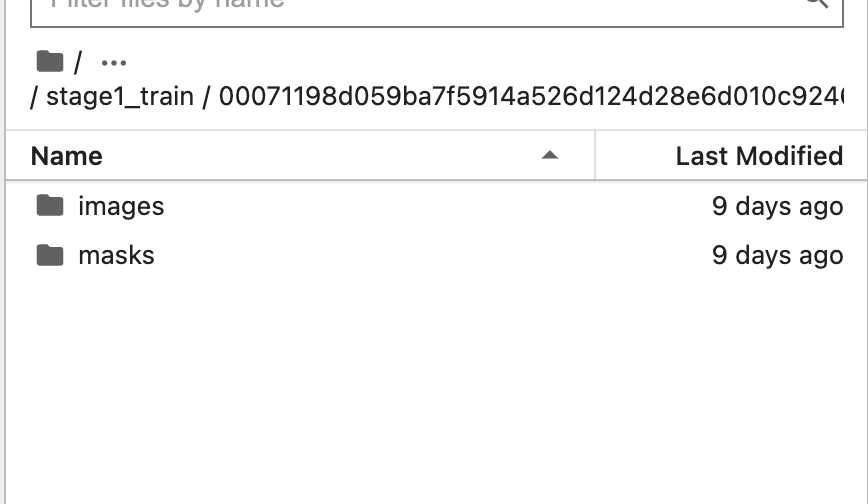
The training data contains images and their corresponding masks. Each image can have multiple masks.

Let's start by creating placeholders for the X and y variables.

# __author__ = "Sreenivas Bhattiprolu"
# https://www.youtube.com/watch?v=0kiroPnV1tM
seed = 42
np.random.seed = seed

IMG_WIDTH = 128
IMG_HEIGHT = 128
IMG_CHANNELS = 3

TRAIN_PATH = 'stage1_train/'
TEST_PATH = 'stage1_test/'

train_ids = next(os.walk(TRAIN_PATH))[1]
test_ids = next(os.walk(TEST_PATH))[1]

X = np.zeros((len(train_ids), IMG_HEIGHT, IMG_WIDTH, IMG_CHANNELS), dtype=np.uint8)
y = np.zeros((len(train_ids), IMG_HEIGHT, IMG_WIDTH, 1), dtype=bool)

Next, resize the training images and create a single image mask for each image from all the available masks.

print('Resizing training images and masks')
for n, id_ in tqdm(enumerate(train_ids), total=len(train_ids)):   
    path = TRAIN_PATH + id_
    img = imread(path + '/images/' + id_ + '.png')[:,:,:IMG_CHANNELS]  
    img = resize(img, (IMG_HEIGHT, IMG_WIDTH), mode='constant', preserve_range=True)
    X[n] = img  #Fill empty X_train with values from img
    mask = np.zeros((IMG_HEIGHT, IMG_WIDTH, 1), dtype=bool)
    for mask_file in next(os.walk(path + '/masks/'))[2]:
        mask_ = imread(path + '/masks/' + mask_file)
        mask_ = np.expand_dims(resize(mask_, (IMG_HEIGHT, IMG_WIDTH), mode='constant',  
                                      preserve_range=True), axis=-1)
        mask = np.maximum(mask, mask_)  
            
    y[n] = mask 

Resize the test images in the same way.  

# test images
test_images = np.zeros((len(test_ids), IMG_HEIGHT, IMG_WIDTH, IMG_CHANNELS), dtype=np.uint8)
sizes_test = []
print('Resizing test images') 
for n, id_ in tqdm(enumerate(test_ids), total=len(test_ids)):
    path = TEST_PATH + id_
    img = imread(path + '/images/' + id_ + '.png')[:,:,:IMG_CHANNELS]
    sizes_test.append([img.shape[0], img.shape[1]])
    img = resize(img, (IMG_HEIGHT, IMG_WIDTH), mode='constant', preserve_range=True)
    test_images[n] = img

print('Done!')

Splitting the training data into a training and validation set will enable the validation of the model's performance later.  

X_train, X_test, y_train, y_test = train_test_split(X, y, test_size=0.33, random_state=42)

Here is a visual of a sample image and its mask image.  

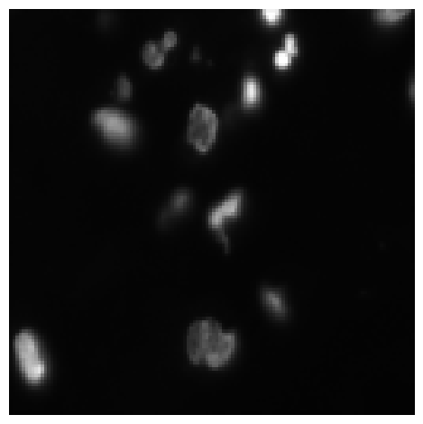
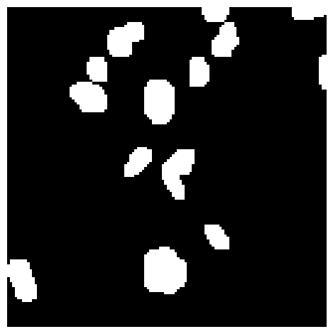
Define Fully Convolutional Network (FCN) in Keras

The Fully Convolutional Network (FCN) will have two main parts:

• The encoder for feature extraction.
• The decoder for upscaling the final feature map to the original image size for segmentation.

Let's start by defining the encoder. You can use an existing CNN network such as VGG; however, in this case, let's design a simple one from scratch.  

Create an input variable that specifies the expected image size. Since this is an FCN, it can accept images of any size. Hence you don't have to specify the size.

inputs = tf.keras.layers.Input(shape=(None, None, 3))

The encoder comprises a stack of convolutional, dropout, and max pooling layers. The model is defined using the Keras Functional API.

def encoder(inputs):
    c1 = tf.keras.layers.Conv2D(16, (3, 3), activation='relu', kernel_initializer='he_normal', padding='same')(inputs)
    c1 = tf.keras.layers.Dropout(0.1)(c1)
    c1 = tf.keras.layers.Conv2D(16, (3, 3), activation='relu', kernel_initializer='he_normal', padding='same')(c1)
    p1 = tf.keras.layers.MaxPooling2D((2, 2))(c1)

    c2 = tf.keras.layers.Conv2D(32, (3, 3), activation='relu', kernel_initializer='he_normal', padding='same')(p1)
    c2 = tf.keras.layers.Dropout(0.1)(c2)
    c2 = tf.keras.layers.Conv2D(32, (3, 3), activation='relu', kernel_initializer='he_normal', padding='same')(c2)
    p2 = tf.keras.layers.MaxPooling2D((2, 2))(c2)

    c3 = tf.keras.layers.Conv2D(64, (3, 3), activation='relu', kernel_initializer='he_normal', padding='same')(p2)
    c3 = tf.keras.layers.Dropout(0.2)(c3)
    c3 = tf.keras.layers.Conv2D(64, (3, 3), activation='relu', kernel_initializer='he_normal', padding='same')(c3)
    p3 = tf.keras.layers.MaxPooling2D((2, 2))(c3)

    c4 = tf.keras.layers.Conv2D(128, (3, 3), activation='relu', kernel_initializer='he_normal', padding='same')(p3)
    c4 = tf.keras.layers.Dropout(0.2)(c4)
    c4 = tf.keras.layers.Conv2D(128, (3, 3), activation='relu', kernel_initializer='he_normal', padding='same')(c4)
    p4 = tf.keras.layers.MaxPooling2D(pool_size=(2, 2))(c4)

    c5 = tf.keras.layers.Conv2D(128, (3, 3), activation='relu', kernel_initializer='he_normal', padding='same')(p4)
    c5 = tf.keras.layers.Dropout(0.2)(c5)
    c5 = tf.keras.layers.Conv2D(128, (3, 3), activation='relu', kernel_initializer='he_normal', padding='same')(c5)
    p5 = tf.keras.layers.MaxPooling2D(pool_size=(2, 2))(c5)

    c6 = tf.keras.layers.Conv2D(256, (3, 3), activation='relu', kernel_initializer='he_normal', padding='same')(p5)
    c6 = tf.keras.layers.Dropout(0.3)(c6)
    c6 = tf.keras.layers.Conv2D(256, (3, 3), activation='relu', kernel_initializer='he_normal', padding='same')(c6)

    u6 = tf.keras.layers.Conv2DTranspose(128, (2, 2), strides=(2, 2), padding='same')(c6)
    c6 = tf.keras.layers.Conv2D(128, (3, 3), activation='relu', kernel_initializer='he_normal', padding='same')(u6)
    c6 = tf.keras.layers.Dropout(0.2)(c6)
    c6 = tf.keras.layers.Conv2D(128, (3, 3), activation='relu', kernel_initializer='he_normal', padding='same')(c6)
    return c6

The decoder will inverse the above convolution process and make predictions for each pixel. Adding the result of the deconvolution and convolution layers improves the segmentation detail.

The final output is obtained by a Conv2D layer with a sigmoid activation and a stride of 1.

num_classes = 1
def decoder(c6):
    u7 = tf.keras.layers.Conv2DTranspose(64, (2, 2), strides=(2, 2), padding='same')(c6)
    c7 = tf.keras.layers.Conv2D(64, (3, 3), activation='relu', kernel_initializer='he_normal', padding='same')(u7)
    c7 = tf.keras.layers.Add()([u7, c7])

    u8 = tf.keras.layers.Conv2DTranspose(32, (2, 2), strides=(2, 2), padding='same')(c7)
    c8 = tf.keras.layers.Conv2D(32, (3, 3), activation='relu', kernel_initializer='he_normal', padding='same')(u8)
    c8 = tf.keras.layers.Add()([u8, c8])

    u9 = tf.keras.layers.Conv2DTranspose(16, (2, 2), strides=(2, 2), padding='same')(c8)
    c9 = tf.keras.layers.Conv2D(16, (3, 3), activation='relu', kernel_initializer='he_normal', padding='same')(u9)
    c9 = tf.keras.layers.Add()([u9, c9])

    u10 = tf.keras.layers.Conv2DTranspose(16, (2, 2), strides=(2, 2), padding='same')(c9)
    c10 = tf.keras.layers.Conv2D(16, (3, 3), activation='relu', kernel_initializer='he_normal', padding='same')(u10)
    c10 = tf.keras.layers.Add()([u10, c10])

    outputs = tf.keras.layers.Conv2D(num_classes, (1, 1), activation='sigmoid')(c10)
    return outputs

It's time to define the Keras model since all the building blocks are ready.

encoder = encoder(inputs)
outputs = decoder(encoder)
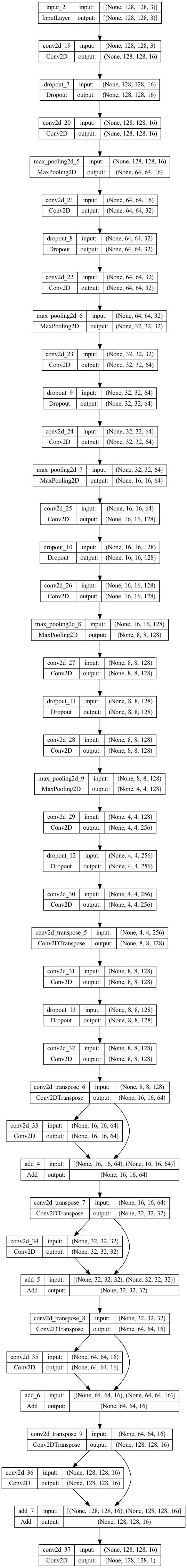
model = tf.keras.Model(inputs=[inputs], outputs=[outputs])

Plotting the FCN model generates the image below.

tf.keras.utils.plot_model(model, "model.png",show_shapes=True)

Train Fully Convolutional Network (FCN) in Keras

Train the model by passing the training and validation data to the Keras fit method. You can also add TensorFlow callbacks such as EarlyStopping to halt training if there is no improvement and the TensorBoard callback to track and visualize the model performance.  

callbacks = [
        tf.keras.callbacks.EarlyStopping(patience=15, monitor='val_loss'),
        tf.keras.callbacks.TensorBoard(log_dir='logs')]

model.fit(X_train, y_train, validation_data=(X_test,y_test), batch_size=16, epochs=100, callbacks=callbacks)

Evaluate Fully Convolutional Network (FCN)

When training is done, you can plot the training and validation loss using Matplotlib.

loss = model.history.history['loss']
val_loss = model.history.history['val_loss']

plt.figure()
plt.plot( loss, 'r', label='Training loss')
plt.plot( val_loss, 'bo', label='Validation loss')
plt.title('Training and Validation Loss')
plt.xlabel('Epoch')
plt.ylabel('Loss Value')
plt.ylim([0, 1])
plt.legend()
plt.show()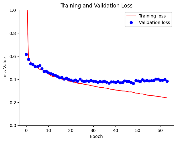

Test Fully Convolutional Network (FCN) on new data

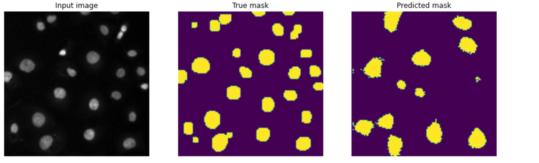
Next, let's test the model's performance on the test images.

def display(display_list):
  plt.figure(figsize=(15, 15))

  title = ['Input image', 'True mask', 'Predicted mask']

  for i in range(len(display_list)):
    plt.subplot(1, len(display_list), i+1)
    plt.title(title[i])
    plt.imshow(tf.keras.utils.array_to_img(display_list[i]))
    plt.axis('off')
  plt.show()
  
 i = random.randint(0, len(X_test))
sample_image = X_test[i]
sample_mask = y_test[i]

prediction = model.predict(sample_image[tf.newaxis, ...])[0]

predicted_mask = (prediction > 0.5).astype(np.uint8)

display([sample_image, sample_mask,predicted_mask])

As you can see from the image below, the model can segment the nuclei. However, it is not very accurate.  

Final thoughts

You have seen how to build a simple segmentation model using Fully Convolutional Neural Networks. The model, however, misses some of the nuclei in the segmentation process. This can be improved by using a model that enables the network to recover more details in the upsampling process. Improving the performance of this model using a different type of neural network will be the subject of my next post.

Meanwhile, check the Kaggle Notebook below to tinker with this model.    

Notebook

Whenever you are ready, there are two ways I can help you:

• Check out my data science and machine learning courses.
• Pick up one of my free or paid data science and machine learning ebooks.

🧡 Enjoy this newsletter?

Forward to a friend and let them know where they can subscribe (hint: it's here).

Anything else? Hit reply to let me know what you think of the post, or say hello.

Join the conversation: Got more questions or comments? Join the conversation in the comments section.

Until next time!