Logistic regression in Python with Scikit-learn

In linear regression, we tried to understand the relationship between one or more predictor variables and a continuous response variable. This article will explore logistic regression, where the response variable will be discrete or categorical.

What is classification?

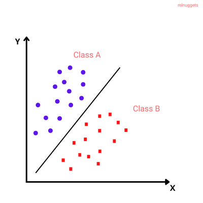
Classification is a supervised machine learning problem of predicting which category or class a particular observation belongs to based on its features.

For instance, one popular classification problem is Image classification. We may want to classify images into different classes: dog, cat, donkey, and human.

Based on pre-classified images of dogs and cats, a classification model can be trained using algorithms like Convolutional Neural Networks (CNN) to classify the images into their respective categories.

There are two types of classification problems:

• Binomial or binary classification: has exactly two classes to choose from.
• Multinomial or Multiclass classification: has three or more classes to choose from.

Some examples of classification algorithms:

• Logistic regression
• Decision trees
• Random forest
• Artificial neural networks
• XGBoost

What is Logistic regression?

Logistic regression is a supervised classification model known as the logit model. It estimates the probability of something occurring, like 'will buy' or 'will not buy,' based on a dataset of independent variables. The outcome should be a categorical or a discrete value. The outcome can be either a 0 and 1, true and false, yes and no, and so on.

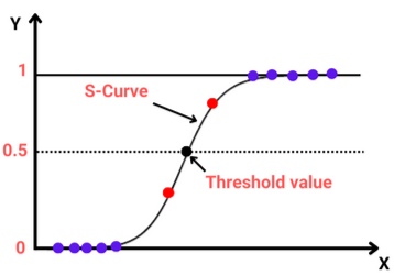
The model does not give an exact 0 and 1 but a value between 0 and 1. Unlike linear regression, which fits a regression line, logistic regression fits an 'S'-shaped logistic function(Sigmoid function).

Logistic function(Sigmoid function)

Since logistic regression is a binary classification technique, the values predicted should fall close to either 0 or 1. This is why a sigmoid function is convenient. In mathematical terms:

Where:

• p(x) is the predicted probability that the output for a given 𝐱 is equal to 1.
• z is the linear function since logistic regression is a linear classifier which translates to:
  • z = b₀ + b₁x₁ + ... + bᵣxᵣ
    Where:
    • b₀, b₁ ...bᵣ are the model's predicted weights or coefficients.
    • x the feature values.

Note that the z can be defined as the log of the probability of something happening(1 = p(x) = will buy) divided by the probability of something not happening(0 = 1-p(x) = will not buy). For this reason, z is referred to as the log-odds or natural logarithm of odds.

The odds mean the probability of success over the probability of failure.

For example, let's imagine we are trying to build a model to predict the probability of a tumor spreading given its size in centimeters. After plotting the dataset, we can use linear regression to model the status p(x) as a function with the sigmoid function.

So let's say after fitting the curve, we get the following values:

• b₀ = -5.47
• b₁ = 1.87

Log-odds would be:

z = -5.47 + (1.87 x 3)

Given a tumor size of 3, we can check the probability with the sigmoid function as:

The probability that the tumor of size 3cm spreads is 0.53, equal to 53%.

Maximum Likelihood Estimation(MLE)

We maximize the log-likelihood function (LLF) to get the best coefficients or the predicted weights. This involves finding the best fit sigmoid curve that provides the optimal coefficients, and this method is called Maximum Likelihood Estimation.

While 𝑦ᵢ = 0, the LLF for that observation is equal to log(1-p(𝐱ᵢ)), and if 𝑝(𝐱ᵢ) is close to 𝑦ᵢ = 0, the log(1-p(𝐱ᵢ)) is close to 0. The main goal is to maximize the LLF. So If 𝑝(𝐱ᵢ) is distant from 0, then the log(1-p(𝐱ᵢ)) drops significantly, and that's not what we want.

Types of logistic regression

So far, we have discussed one type of binary type of logistic regression where the outcome is a 0/1, True/False, and so on. There are two more types:

• Multinomial logistic regression: This type of regression has three or more unordered types of dependent variables, such as cats/dogs/donkeys.
• Ordinal logistic regression: Has three or more ordered dependent variables such as poor/average/ good or high/medium/average.

Assumptions of logistic regression

Logistic regression assumes that:

• The response variable is binary or dichotomous.
• The observations or independent variables have very little or no multicollinearity.
• There are no extreme outliers.
• There is a linear relationship between the predictor variables and the log-odds of the response variable.
• Large sample sizes for a more reliable analysis.

Logistic regression with Scikit-learn

To implement logistic regression with Scikit-learn, you need to understand the Scikit-learn modeling process and linear regression.

The steps for building a logistic regression  include:

• Import the packages, classes, and functions.
• Load the data.
• Exploratory Data Analysis(EDA).
• Transform the data if necessary.
• Fit the classification model.
• Evaluate the performance model.

Importing packages

First, you need to import Seaborn for visualization, NumPy, and Pandas. In addition, import:

• LogisticRegression for fitting the model.
• confusion_matrix and classification_report for evaluating the model.  

import numpy as np
import pandas as pd
import matplotlib.pyplot as plt
import seaborn as sns
from sklearn.linear_model import LogisticRegression
from sklearn.metrics import confusion_matrix, classification_report

Loading the dataset

Import the  Social Network Ads dataset from Kaggle. The data is a CSV file with data that will help us build a logistic regression model to show which users purchased or did not purchase a product.

social_N_data = pd.read_csv('Social_Network_Ads.csv')
pd.concat([social_N_data.head(), social_N_data.tail()])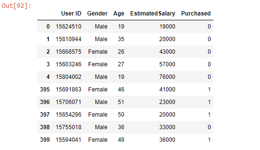

Exploratory Data Analysis

Analyzing the data first is key to understanding its characteristics. We will begin with checking the missing values.

social_N_data.isnull().any()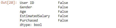

No null values in the dataset.

Check for the total number of those who purchased and those who did not purchase:

sns.countplot(x='Purchased', data=social_N_data)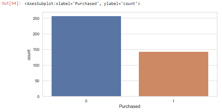

Zero indicates those who did not purchase and 1 for those who bought.

Check for how many males and females purchased the product:

sns.countplot(x='Purchased', hue='Gender', data=social_N_data)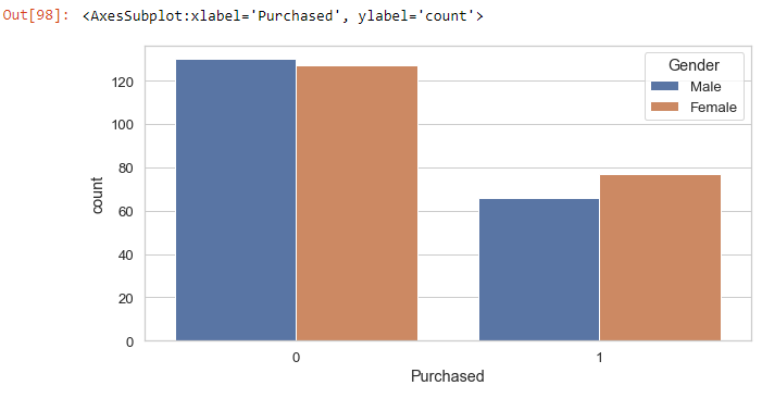

From the plot, we can see that most people who did not purchase are male, and the majority of those who purchased are female.

We can also check the age distribution in the dataset:

sns.displot(x='Age', data=social_N_data, color='red', kde=True)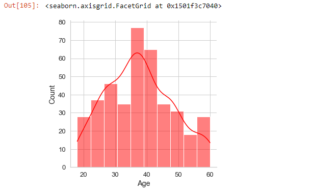

Cleaning the data

We will use the Gender, Age, and EstimatedSalary columns from the dataset for the logistic regression. This means that we do not require the UserID column. Thus we will drop it.

social_N_data.drop('User ID', axis=1, inplace=True)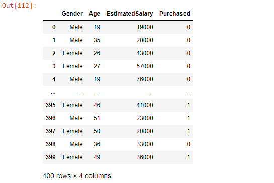

Changing categorical data into dummies

Let's look at the info of the dataset to get a general idea of what it contains.

social_N_data.info()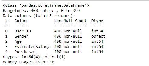

The Gender variable is categorical. For the model to work, we will convert it into dummy variables using the Pandas get_dummies or the oneHotEncodermethod.

Change Gender to dummy variable and drop the first dummy to prevent multicollinearity:

gender = pd.get_dummies(social_N_data['Gender'], drop_first=True)

social_N_data.drop('Gender',axis=1,inplace=True)

social_N_data = pd.concat([social_N_data,gender], axis=1)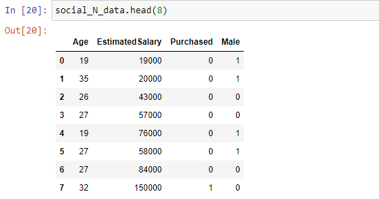

When the Male value is 1, it means the gender is male, and when the value is 0, the gender is female. We did not require both the Female and Gender variables in the dataset, as one can be used to predict the other.

Splitting the data into independent(X) and dependent(y) variables

Split the data into independent and dependent variables.

X = social_N_data.iloc[:,[0,1,3]] # Age, EstimatedSalary and Male
X.head()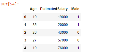

y = social_N_data.iloc[:, 2] # Purchased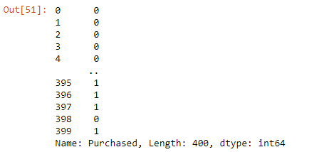

Feature scaling

Feature scaling is a method used to normalize the range of independent variables. The method enables the independent variables to be in the same range.

When working with large datasets, scaling plays a significant role in improving the performance of the model.

In the data, we will import the StandardScaler from Scikit-learn preprocessing module and use it to transform the data. For instance, there is a big difference between the values of the Age variable and those of EstimatedSalary.

from sklearn.preprocessing import StandardScaler
sc = StandardScaler()
X = sc.fit_transform(X)
X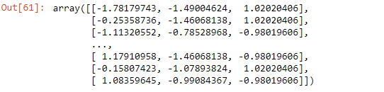

Splitting the dataset into train and test sets

Split the dataset into training and testing sets using the train_test_split function.

from sklearn.model_selection import train_test_split 
X_train, X_test, y_train, y_test = train_test_split(X, y, test_size=0.30, random_state=1)

print(X_train.shape)
print(X_test.shape)
print(y_train.shape)
print(y_test.shape)

'''
(280, 3)
(120, 3)
(280,)
(120,)
'''

Fitting the logistic regression model and predicting test results

Now that the dataset is well prepared, we can train the model by importing the LogisticRegression class of the Scikit-learn linear_model module.

Training is done by calling the fit method and pass the training data.

from sklearn.linear_model import LogisticRegression  
classifier = LogisticRegression()
classifier.fit(X_train, y_train)

The model is now trained on the training set. Let's perform prediction on the test set using the predict method.

y_pred = classifier.predict(X_test)

Let's create a Pandas DataFrame and compare the predicted and actual values.  

result = pd.DataFrame({'Actual' : y_test, 'Predicted' : y_pred})
result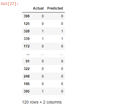

The coef_ and intercept_ attributes give the model coefficient and intercept.

classifier.coef_
# array([[2.36839196, 1.42929561, 0.20973787]])
classifier.intercept_ 
# array([-1.1352347])

Evaluating the model

There are various ways of checking the performance of the model.

Using predict_proba

It returns the matrix of probabilities that the predicted output is equal to zero or one.

print(classifier.predict_proba(X))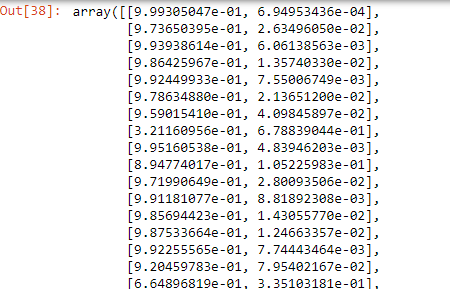

From the matrix, each row represents a single observation. The first column is the probability that the product is not purchased(1-p(x)), and the second column is the probability that the product is purchased(p(x)).

Using confusion matrix

From the Scikit-learn metrics module, we import confusion_matrix. The confusion matrix is the number of correct and incorrect predictions column-wise, showing the following values:

• True negatives(TN) in the upper-left position.
• False negatives(FN) in the lower-left position.
• False positives(FP) in the upper-right position.
• True positives(TP) in the lower-right position.

from sklearn.metrics import confusion_matrix
cf_matrix = confusion_matrix(y_test, y_pred)
cf_matrix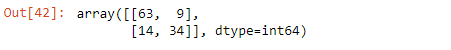

The output of the confusion matrix is a 2*2 matrix since the model is a binary classification. Let's visualize it better using a heatmap and explain.

sns.heatmap(pd.DataFrame(cf_matrix), annot=True, cmap="YlGnBu" ,fmt='g')
plt.title('Confusion matrix', y=1.1)
plt.ylabel('Actual label')
plt.xlabel('Predicted label')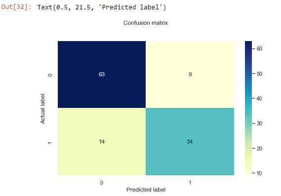

From the confusion_matrix, we have the following observations:

• 63 TN predictions: zeros predicted correctly.
• 14 FN predictions: ones wrongly predicted as zeros.
• 9 FP predictions: zeros that were wrongly predicted as ones.
• 34 TP predictions: ones predicted correctly.

To calculate the model's accuracy from the confusion matrix, we divide the sum of TN and TP by the sum of all the predictions.

Accuracy = (63 + 34)/(63 + 34 + 9 + 14)
Accuracy
# 0.8083333333333333

# Also same result from sklearn accuracy_score
from sklearn.metrics import accuracy_score

accuracy_score(y_test,y_pred)
#0.8083333333333333

The accuracy of our model is about 80% which is ideal.

Confusion matrix metrics

The classification_report gives a more comprehensive report of the model's performance.

target_names = ['will NOT PURCHASE', 'will PURCHASE']
print(classification_report(y_test, y_pred,target_names=target_names))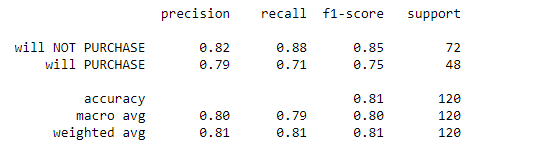

Complete code for logistic regression

import numpy as np
import pandas as pd
import matplotlib.pyplot as plt
import seaborn as sns
from sklearn.preprocessing import StandardScaler
from sklearn.model_selection import train_test_split 
from sklearn.linear_model import LogisticRegression
from sklearn.metrics import confusion_matrix, classification_report, accuracy_score

social_N_data = pd.read_csv('Social_Network_Ads.csv')
pd.concat([social_N_data.head(), social_N_data.tail()])

#CHECK FOR NULL VALUES
social_N_data.isnull().any()

# CLEAN THE DATA
social_N_data.drop('User ID', axis=1, inplace=True)

# CHANGE CATEGORICAL VARIABLE TO DUMMIES
social_N_data.info()
gender = pd.get_dummies(social_N_data['Gender'], drop_first=True)
social_N_data.drop('Gender',axis=1,inplace=True)
social_N_data = pd.concat([social_N_data,gender], axis=1)

# SPLIT DATA TO INDEPENDENT AND DEPENDENT VARIABLES
X = social_N_data.iloc[:,[0,1,3]] # Age, EstimatedSalary and Male
y = social_N_data.iloc[:, 2] # Purchased

# FEATURE SCALING
sc = StandardScaler()
X = sc.fit_transform(X)

# SPLIT DATA TO TRAIN AND TEST SET
X_train, X_test, y_train, y_test = train_test_split(X, y, test_size=0.30, random_state=1)

# FIT/TRAIN MODEL
classifier = LogisticRegression()
classifier.fit(X_train, y_train)

# PREDICTIONS
y_pred = classifier.predict(X_test)
result = pd.DataFrame({'Actual' : y_test, 'Predicted' : y_pred})
print(result)

# EVALUATE MODEL
# predic_proba()
# print(classifier.predict_proba(X) # uncheck if needed
#confusion matrix
cf_matrix = confusion_matrix(y_test, y_pred)
print('Confusion Matrix \n', cf_matrix)

sns.heatmap(pd.DataFrame(cf_matrix), annot=True, cmap="YlGnBu" ,fmt='g')
plt.title('Confusion matrix', y=1.1)
plt.ylabel('Actual label')
plt.xlabel('Predicted label')

print('Accuracy of model')
print(accuracy_score(y_test,y_pred) * 100, '%')
#0.8083333333333333

# classification report
target_names = ['will NOT PURCHASE', 'will PURCHASE']
print('Classification report: \n', classification_report(y_test, y_pred,target_names=target_names))

Final thoughts

Logistic regression is direct and friendly to implement. Hopefully, you can now analyze various datasets using the logistic regression technique. Generally, we have covered:

• Logistic regression in relation to the classification.
• Logistic or Sigmoid function.
• How logistic regression uses MLE to predict outcomes.
• Assumptions of logistic regression.
• Step-by-step implementation of logistic regression.

The Complete Data Science and Machine Learning Bootcamp on Udemy is a great next step if you want to keep exploring the data science and machine learning field.

Follow us on LinkedIn, Twitter, and GitHub, and subscribe to our blog, so you don't miss a new issue.