How to create custom training loops in Keras

Training models in Keras is usually done using the fit method. However, you may want more control over the training process. To do that, you'll need to create a custom training loop. This involves setting up a custom function to compute the loss and gradient. This article will walk you through the process of doing that. Let's get to it.

Obtain dataset

We'll use the Fashion MNIST dataset for this illustration and load it using the Layer data loader.

# pip install layer
import layer
mnist_train = layer.get_dataset('layer/fashion_mnist/datasets/fashion_mnist_train').to_pandas()
mnist_test = layer.get_dataset('layer/fashion_mnist/datasets/fashion_mnist_test').to_pandas()
# Successfully logged into https://app.layer.ai as guest
# ⠴  fashion_mnist_train  ━━━━━━━━━━ LOADED [0:00:10] 
# ⠦  fashion_mnist_test   ━━━━━━━━━━ LOADED [0:00:04] 

Here's is how the dataset looks like:

mnist_train["images"][17]
mnist_test["images"][23]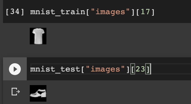

Data processing

Next, convert the cloth images to NumPy arrays.

import numpy as np
def images_to_np_array(image_column):
    return np.array([np.array(im.getdata()).reshape((im.size[1], im.size[0])) for im in image_column])
train_images = images_to_np_array(mnist_train.images)
test_images = images_to_np_array(mnist_test.images)
train_labels = mnist_train.labels
test_labels = mnist_test.labels

Scaling data in deep learning is a common practice because weights and biases of the network are initialized to small numbers between 0 and 1. We, therefore, have to scale the image data.

train_images = train_images / 255.0
test_images = test_images / 255.0
train_images.shape
# (60000, 28, 28)

The neural network expects the above dataset to be in a specific shape. When training models with Keras, we pass the shape as image_width, image_height , number_of_channels. In the shape printed above, we see that the number_of_channels is missing. We need to add that. Failure to do this will result in an error similar to:

ValueError: Exception Input 0 of layer "conv2d" is incompatible with the layer: expected min_ndim=4, found ndim=3. 

To avoid that, expand the dimensions.

# Make sure images have shape (28, 28, 1)
train_images = np.expand_dims(train_images, -1)
test_images = np.expand_dims(test_images, -1)
train_images.shape
# (60000, 28, 28, 1)

Batch the dataset

Next, let's define the number of images that will be passed to the network. 32 is a common choice, but this number can be changed. Let's create batches out of the training images. Passing images in batches also makes training faster. We start by creating a tf.dataset with the from_tensor_slices method, then add the batch size.  

ds_train_batch = tf.data.Dataset.from_tensor_slices((train_images, train_labels))
training_data = ds_train_batch.batch(32)
ds_test_batch = tf.data.Dataset.from_tensor_slices((test_images, test_labels))
testing_data = ds_test_batch.batch(32)

How to create model with custom layers in Keras

Custom layers in TensorFlow are created by inheriting tf.keras.Layer and implementing __init__, build and call.

class MyDenseLayer(tf.keras.layers.Layer):
  def __init__(self, num_outputs):
    super(MyDenseLayer, self).__init__()
    self.num_outputs = num_outputs

  def build(self, input_shape):
    self.kernel = self.add_weight("kernel",
                                  shape=[int(input_shape[-1]),
                                         self.num_outputs])

  def call(self, inputs):
    return tf.matmul(inputs, self.kernel)

layer = MyDenseLayer(10)

A better way to create custom layers is to inherit keras.Model because it avails the Model.fit,Model.evaluate, and Model.save methods. Let's create a custom block with the following layers:

• Convolution.
• Max pooling.
• Flatten.
• DropOut.
• Dense.

parameters = {"shape":28, "activation": "relu", "classes": 10, "units":12, "optimizer":"adam", "epochs":100,"kernel_size":3,"pool_size":2, "dropout":0.5}

class CustomBlock(tf.keras.Model):
  def __init__(self, filters):
    super(CustomBlock, self).__init__(name='')
    filters1, filters2 = filters
    self.conv2a = layers.Conv2D(filters=filters1,input_shape=(28,28,1), kernel_size=(parameters["kernel_size"], parameters["kernel_size"]), activation=parameters["activation"])

    self.maxpool1a = layers.MaxPooling2D(pool_size=(parameters["pool_size"], parameters["pool_size"]))

    self.conv2b = layers.Conv2D(filters2, kernel_size=(parameters["kernel_size"], parameters["kernel_size"]), activation=parameters["activation"])

    self.maxpool2b = layers.MaxPooling2D(pool_size=(parameters["pool_size"], parameters["pool_size"]))

    self.flatten1a = layers.Flatten()
    self.dropout1a = layers.Dropout(parameters["dropout"])
    self.dense1a = layers.Dense(parameters["classes"], activation="softmax")

  def call(self, input_tensor):
    x = self.conv2a(input_tensor)
    x = tf.nn.relu(x)
    x = self.maxpool1a(x)

    x = self.conv2b(x)
    x = tf.nn.relu(x)
    x = self.maxpool2b(x)

    x = self.flatten1a(x)
    x = self.dropout1a(x)
    x = self.dense1a(x)
    return tf.nn.softmax(x)

Let's initialize the model and check the layers and variables.  

model = CustomBlock([32,64])
input_shape = (1, 28, 28, 1)
x = tf.random.normal(input_shape)
_ = model(x)
x.shape
# TensorShape([1, 28, 28, 1])
model.layers
len(model.variables)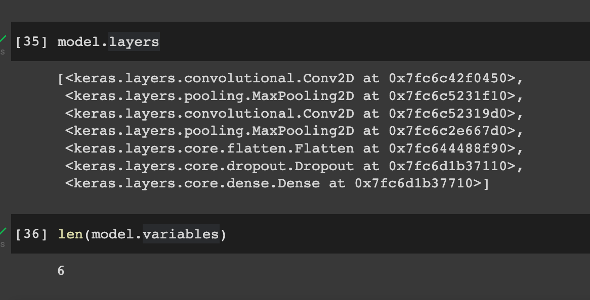

We can also visualize the model's summary.

model.summary()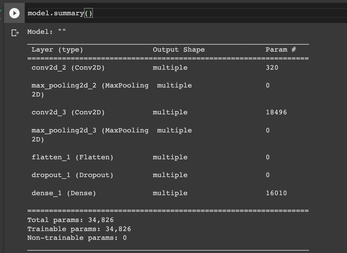

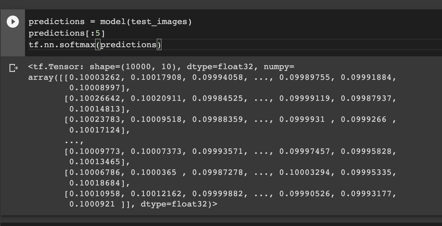
The model can be used to make predictions even before training. Obviously, the results won't be good.

Define the loss  function

The next step is to define the loss function. We use  SparseCategoricalCrossentropy because the labels are integers. If labels are one-hot encoded  CategoricalCrossentropy is used instead. The goal is to reduce the errors between the true and predicted values. The SparseCategoricalCrossentropy function takes probability predictions and returns the average loss.

loss_object = tf.keras.losses.SparseCategoricalCrossentropy()
def loss(model, x, y, training):
  # training=training is needed only if there are layers with different
  # behavior during training versus inference (e.g. Dropout).
  y_ = model(x, training=training)

  return loss_object(y_true=y, y_pred=y_)

l = loss(model, test_images, test_labels, training=False)
print("Loss test: {}".format(l))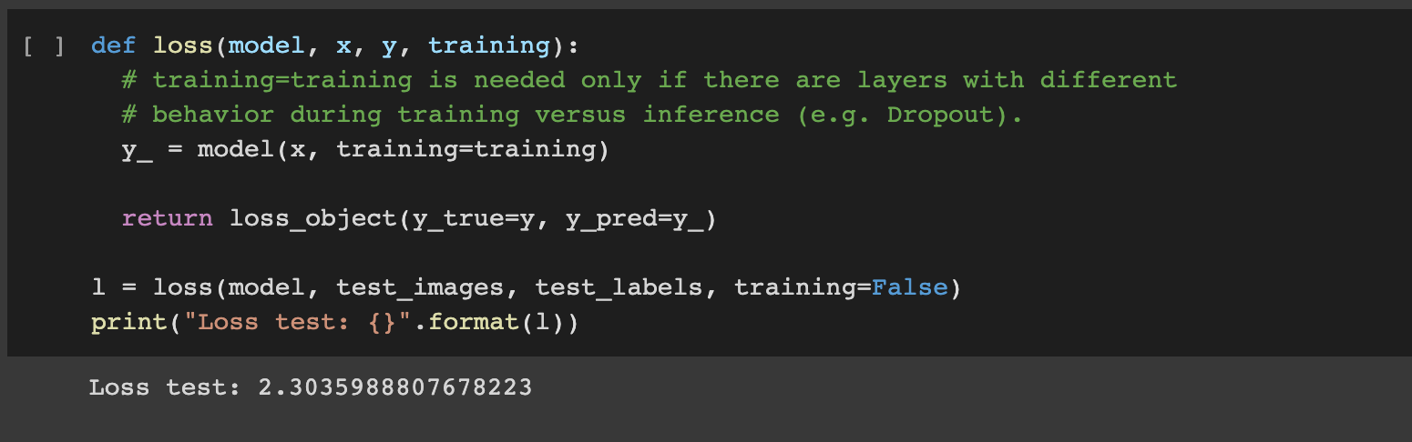

Define the  gradients function

The gradient is computed using the tf.GradientTape function. It calculates the gradient of the loss with respect to the model trainable variables. The tape records operations in the forward pass and uses this information to compute gradients on the backward pass.

def grad(model, inputs, targets):
  with tf.GradientTape() as tape:
    loss_value = loss(model, inputs, targets, training=True)
  return loss_value, tape.gradient(loss_value, model.trainable_variables)

Create an optimizer

An optimizer function uses the computed gradients to adjust the model weights and biases to minimize the loss. This iterative process aims to find the model parameters that result in the least error. We apply the common Adam optimizer function.

optimizer = tf.keras.optimizers.Adam()

Create custom training loop

The training loop feeds the training images to the network while computing the metrics. We use the SparseCategoricalAccuracy to compute the accuracy because the labels are integers. If labels are one-hot encoded, the CategoricalAccuracy is used. We use tqdm to display a progress bar of the training process. The training process involves the following steps:

• Pass the training data to the network for one epoch.
• Obtain the training images and labels for each batch.
• Run predictions using the network and compare the result with the true values.
• Update model parameters using the Adam optimizer.
• Track the training metrics for visualization later.
• Repeat the process for the specified number of epochs.    

from tqdm.notebook import trange
## Note: Rerunning this cell uses the same model parameters

# Keep results for plotting
train_loss_results = []
train_accuracy_results = []

num_epochs = 10

for epoch in trange(num_epochs):
  epoch_loss_avg = tf.keras.metrics.Mean()
  epoch_accuracy = tf.keras.metrics.SparseCategoricalAccuracy()

  # Training loop - using batches of 32
  for x, y in training_data:
    # Optimize the model
    loss_value, grads = grad(model, x, y)
    optimizer.apply_gradients(zip(grads, model.trainable_variables))

    # Track progress
    epoch_loss_avg.update_state(loss_value)  # Add current batch loss
    # Compare predicted label to actual label
    # training=True is needed only if there are layers with different
    # behavior during training versus inference (e.g. Dropout).
    epoch_accuracy.update_state(y, model(x, training=True))

  # End epoch
  train_loss_results.append(epoch_loss_avg.result())
  train_accuracy_results.append(epoch_accuracy.result())
  print("Epoch {}: Loss: {:.3f}, Accuracy: {:.3%}".format(epoch + 1,
                                                                epoch_loss_avg.result(),
                                                                epoch_accuracy.result()))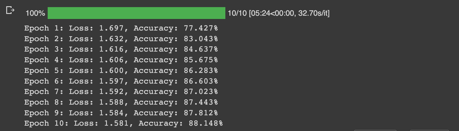

Visualize the loss

Next, visualize the training loss and accuracy with Matplotlib.

fig, axes = plt.subplots(2, sharex=True, figsize=(12, 8))
fig.suptitle('Training Metrics')

axes[0].set_ylabel("Loss", fontsize=14)
axes[0].plot(train_loss_results)

axes[1].set_ylabel("Accuracy", fontsize=14)
axes[1].set_xlabel("Epoch", fontsize=14)
axes[1].plot(train_accuracy_results)
plt.show()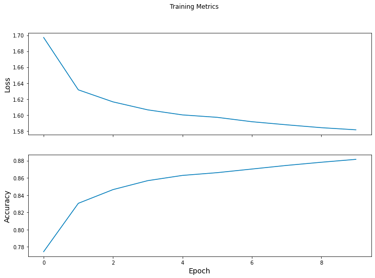

Read more: TensorBoard tutorial (Deep dive with examples and notebook)

Evaluate model on test dataset

To evaluate the network's performance, we loop through the test data, make predictions and compare them with the true values.  tf.math.argmax returns the axis of the largest predicted value.

test_accuracy = tf.keras.metrics.Accuracy()

for (x, y) in testing_data:
  # training=False is needed only if there are layers with different
  # behavior during training versus inference (e.g. Dropout).
  logits = model(x, training=False)    
  prediction = tf.math.argmax(logits, axis=1, output_type=tf.int64)
  test_accuracy(prediction, y)
print("Test set accuracy: {:.3%}".format(test_accuracy.result()))
# Test set accuracy: 87.870%

Use the trained model to make predictions

Let's use the trained model to make predictions on new cloth images and print the prediction. The model outputs logits which we pass to the tf.nn.softmax. This ensures that the sum of all the outputs sums to 1. We, therefore, take the maximum value as the predicted value. Obtaining the index of the maximum and mapping it to categories gives the predicted class.

# training=False is needed only if there are layers with different
# behavior during training versus inference (e.g. Dropout).
predictions = model(test_images[0:5], training=False)
class_names = ["T-shirt/top","Trouser","Pullover","Dress","Coat","Sandal","Shirt","Sneaker","Bag","Ankle boot"]
for i, logits in enumerate(predictions):
  class_idx = tf.math.argmax(logits).numpy()
  p = tf.nn.softmax(logits)[class_idx]
  name = class_names[class_idx]
  print("Image {} prediction: {} ({:4.1f}%)".format(i, name, 100*p))

Final thoughts

You have now learned to create custom layers and training loops in Keras. This helps understand the underlying processing that happens when you call the fit method from Keras. It's also important if you want more fine-grained control of the network's training process. Specifically, we have seen that creating custom training loops involves:

• Design the network using custom layers or using the Keras built-in layers.
• Creating custom loss functions.
• Building a custom function to compute model gradients.
• Defining the optimizer function.    
• Creating the custom loop function that utilizes the loss and gradient functions.

TensorFlow resources

Object detection with TensorFlow 2 Object detection API

How to train deep learning models on Apple Silicon GPU

How to build CNN in TensorFlow(examples, code, and notebooks)

How to build artificial neural networks with Keras and TensorFlow

The Complete Data Science and Machine Learning Bootcamp on Udemy is a great next step if you want to keep exploring the data science and machine learning field.

Follow us on LinkedIn, Twitter, GitHub, and subscribe to our blog, so you don't miss a new issue.