Transfer learning guide(With examples for text and images in Keras and PyTorch)

Training computer vision (CV) or natural language processing (NLP) models can be expensive and requires large datasets. If labeling is done manually, the process will take a longer training time and requires expensive hardware.

For instance, the Generative Pre-trained Transformer 2 (GPT-2), a benchmark-setting language model created by Open AI in 2019, is estimated to have cost around $1.6m to train. Such a cost would make it difficult for individuals or small organizations conducting research in NLP to compete with Open AI.

Luckily, you do not have to train models such as GPT-2. You can obtain a copy of such models free of charge from the internet, fine-tune them to match your requirements and specific dataset, and obtain results faster.

In this guide, we will explore the concept of transfer learning and its applications in computer vision and natural language processing.

What is transfer learning?

Transfer learning is the process where a model built for a problem is reused for a different or similar task. This technique is commonly used in computer vision and natural language processing, where previously trained models are used as the base for new related problems to save time.

The pre-trained base models are trained on large benchmark datasets in computer vision and natural language processing. The resulting weights are used on another task with a smaller set of data.

This approach not only reduces training time but also lowers the generalization error. The figure below depicts the transfer learning idea.

Advantages of using pre-trained models

The main advantage of using pre-trained models is their general adaptability for use in other real-world applications. For example:

• For problems that require researchers to build models but face downstream requirements including latency constraints or specific data domains, models such as GAIA and COCO trained on ImageNet can be used effectively.
• In NLP, classifying text data requires knowledge of word representations in some vector space. Training custom representations is feasible, except that you might not have sufficient data to train the embeddings. In such cases, pre-trained word embeddings like Word2Vec and GloVe, are used to speed up the modeling process.

Types of transfer learning

Transfer learning can be categorized into three groups depending on the machine learning model involved.

Inductive transfer learning

In inductive transfer learning, the source and target domains are the same. However, the source and target problems vary. The models use the knowledge and inductive biases of the source (base) model to improve the target problem.

Inductive transfer learning can be grouped into two subcategories, i.e., multitask learning and self-taught learning. The pre-trained model already has domain features and is a better starting point than training the model from scratch.

Inductive transfer learning involves extending well-known classification and inference models, including neural networks, Bayesian networks, and Markov Logic Networks.

Unsupervised transfer learning

Unsupervised transfer learning focuses on unsupervised tasks in the target domain where the source and target domains are similar, but the problems differ. In this case, the data in either domain is not labeled.

In unsupervised and semi-supervised settings, transfer learning assumes that a reasonably sized dataset exists in the target task, but it is generally unlabeled, following the expense of having an individual assign the labels manually.

Transductive transfer learning

In transductive transfer learning, the domains of the source and target problems are not exactly similar but have interrelated uses. One can derive similarities between the source and target tasks.

These settings generally use a lot of labeled data in the source domain, whereas the target domain contains only unlabeled data. Transductive transfer learning can be grouped into subcategories, depending on whether the feature spaces are different or the marginal probabilities.

Further, transfer learning can be categorized depending on the similarity between the domain and independence of the type of data samples used for training, i.e., homogeneous and heterogeneous transfer learning.

Homogeneous transfer learning

Homogeneous transfer learning techniques are created and used to handle scenarios where the domains originate from the same feature space. In this transfer learning technique, the domains slightly differ in marginal distributions.

These techniques adapt the domains by correcting the sample selection bias or covariate shift. Examples of homogeneous transfer learning include instance, parameter, and relational-knowledge transfer.

Heterogeneous transfer learning

Heterogeneous transfer learning techniques derive representations from a pre-trained network to obtain meaningful features from new samples for a closely related task. Nonetheless, these techniques do not account for the existing difference in the feature spaces of source and target domains.

It is time-consuming and expensive to collect labeled source data with the same feature space as the target domain. In such cases, heterogeneous transfer learning techniques address such constraints.

Heterogeneous transfer learning addresses the problem of the source and target domains containing different feature spaces and other issues such as different data distributions and label spaces. This type of transfer learning is prevalent in cross-domain problems like cross-language text categorization, text-to-image classification, etcetera.

What is the difference between transfer learning and fine-tuning?

Transfer learning is a setting where weights obtained in one problem– e.g., on a large-scale image classification task– are exploited to improve generalization in another problem (say, fruit classification) without having to train the models from scratch.

Fine-tuning is an optional step in transfer learning used to improve the model's performance. This step usually involves adapting the pre-trained model to a particular task or problem.

However, since the entire model has to be re-trained, it is likely to overfit. Overfitting fine-tuned models can be solved by re-training the model or part of it using a low learning rate to prevent significant updates to the gradient, which results in poor predictive performance.

Applying a callback to stop the training process when the model's performance is not improving is also helpful for obtaining better weights.

Other approaches to prevent overfitting include:

• Increasing the batch size.
• Using different regularization techniques.

Why use transfer learning?

Training neural network models require a lot of data which is not always available. On top of that, you need resources such as infrastructure to train the models.

Transfer learning offers numerous advantages. Reducing training time because training large models can take several days or weeks is key among them.

When do you use transfer learning?

Transfer learning is mainly used when:

• There isn't enough labeled data to train the model.
• An existing pre-trained model has already been trained on similar data and problems– avoid reinventing the wheel.
• If you have trained an initial model, you might restore it and re-train some layers for a new problem.

When does transfer learning not work?

Even though transfer learning has transformed model development in computer vision and natural language processing domains, the process might fail sometimes. In other cases, you might end up with modest results. Such cases occur when there is dissimilarity in datasets and domains.

There is a significant relationship between domain divergence and transfer learning performance. Different transfer learning strategies and techniques are applied based on the domain of the application, the problem at hand, and the available data. Therefore, using a pre-trained model from a different domain on an unrelated problem or unrelated data might underperform or fail altogether because features transfer poorly.

For instance, training a DenseNet model on ImageNet and using it to fine-tune on a medical dataset. Another case is using a pre-trained GPT model on WikiText 103 for the medical articles dataset. To solve this, do domain adaption first and then train the models on the target task to improve performance.

Another dissimilarity could be related to variations in the dimension of the inputs from these datasets. For instance, using a pre-trained ResNet for CIFAR-10 (32x32px) to fine-tune on MNIST Handwritten Digit Classification (28x28px).

How to implement transfer learning?

Transfer learning involves taking features from one task and using them on a similar task. For instance, features from a model trained to identify rats may be useful as a base model trained to identify mice. This section will go through the process of implementing transfer learning.

Transfer learning in 6 steps

The process of implementing transfer learning follows six major steps, as shown below:

A pre-trained model can be used directly to classify new images as one of the 1,000 known classes included in the image classification task in the ILSVRC (ImageNet).

A sample transfer learning using a model trained on the ImageNet dataset and used on a smaller data set, i.e., the food dataset, is shown below.

Step 1: Obtain the pre-trained model

After determining the suitable model for your problem, the next step involves acquiring the model. More about this later in the article.

Most pre-trained models have different architectures. Neural network architectures fall into two main groups, i.e., supervised learning, where the data used for training is labeled, and unsupervised learning, where the data is unlabeled. The main architectures for supervised learning include Convolutional Neural Networks (CNNs) and Recurrent Neural Networks (RNNs).

Step 2: Create a base model

The initial step in each transfer learning task involves instantiating the base model using a preferred architecture such as VGG or ResNet with or without pre-trained weights. Failure to download the weights means that the model will be trained from scratch.

Since the dataset used to train the base model contains a superset of the labels in your dataset, it tends to have more units in the final output layer than you need. You will have to drop the final output layer and incorporate a final output layer compatible with your task.

Step 3: Freeze layers so they don’t change during training

In most cases, your dataset will be small. In this scenario, you can freeze the initial (let's say k) layers of the pre-trained model and train a new model with the remaining(n-k) layers.

Freezing layers prevents the weights in those layers from being re-initialized since they will lose all the learned information, which will be the same as training a new model from scratch.

To prevent re-initialization of weights, specify the base model to be non-trainable.

base_model.trainable = False

Or using:

base_model.trainable = 0

Step 4: Add new trainable layers

We are only using the feature extraction layers from the base model. It is important to include additional layers on top of the frozen layers to learn new weights and features for the new specialized tasks. The added layers are generally the final output layers excluded from the base model.

Step 5: Train the new layers on the dataset

Include a dense output layer that contains units corresponding to the number of outputs expected by the model. For example, the final dense layer should represent the class scores in the food classification problem.

Step 6: Improve the model via fine-tuning

Fine-tuning aims to improve the performance of the model. It is done by unfreezing the entire base model or part of it and then re-training the resulting model on the whole dataset using a relatively low learning rate.

Setting a low learning rate for the model will prevent overfitting while improving the model's performance on the new problem.

Recall that the original model was defined with many parameters fit for the large dataset. Therefore, it is essential to have a very low learning rate because you are training the original model on a smaller dataset. Failure to do this will lead to overfitting.

When using the base model with frozen layers, the model's behavior is also frozen during the execution of the compile function. As such, you will need to execute the compile function again whenever any changes are made to the model for the model's behavior to adapt to the new changes.

After making the changes, compile the resulting model to allow the changes to take effect. Subsequently, you will train the model again while monitoring it using callbacks to prevent the model from overfitting.

Where to find pre-trained models?

Pre-trained models can be obtained from the internet through various sources, including:

• Keras applications
• Tensorflow Hub
• PyTorch Hub

In this section, we will explore how to fetch pre-trained models.

Keras pre-trained models

Keras provides access to approximately 35 fully-trained convolutional neural networks. Currently, the EfficientNetV2Larchitecture has the highest top accuracy, i.e., 97.5%, while MobileNet has the least top accuracy, i.e., 89.5%.

You can select any model for your problem. Once you have downloaded a pre-trained model, you obtain the pre-trained weights. Both are stored in the ~/.keras/models/ directory.

The following example demonstrates how to instantiate the smaller version ofMobileNetV2 architecture trained on ImageNet.

import tensorflow as tf
IMAGE_SIZE = 224 # define images size
pretrained_model = tf.keras.applications.MobileNetV3Small(
    input_shape = (IMAGE_SIZE, IMAGE_SIZE, 3),
    alpha=1.0,
    include_top=True,
    weights="imagenet",
    input_tensor=None,
    pooling=None,
    classes=1000,
    classifier_activation="softmax"
)
#
pretrained_model.trainable = False
#summary of the architecture
pretrained_model.summary()

Transfer learning using TensorFlow Hub

You can also obtain pre-trained models from the TensorFlow Hub, which lets you search and access hundreds of trained, ready-to-deploy machine learning models in one place. Sticking to the smaller version ofMobileNetV2 architecture, you can obtain it from TensorFlow Hub, as shown below:

import tensorflow as tf
import tensorflow_hub as hub
#link to the pre-trained model
mobilenet_v2 ="https://tfhub.dev/google/imagenet/mobilenet_v3_small_100_224/classification/5"
#define the model name you want to acquire
classifier_model = mobilenet_v2

IMAGE_SHAPE = 224

classifier = tf.keras.Sequential([
    hub.KerasLayer(classifier_model, 
    input_shape=(IMAGE_SHAPE, IMAGE_SHAPE, 3))
	])
classifier.summary()

Pretrained word embeddings

In NLP applications, the goal is to generate a representation of words that store their meanings, semantic associations, and the different types of contexts in which they are applied in. These representations are referred to as word embeddings.  

Some sources for pre-trained word embeddings include:

• Stanford’s GloVe pre-trained word embeddings
• Google’s Word2vec
• Fasttext

Stanford’s GloVe pre-trained word embeddings

Below is an example of an implementation for the GloVe pre-trained word embeddings.

# download glove and unzip it in Notebook.
!wget http://nlp.stanford.edu/data/glove.6B.zip
!unzip glove*.zip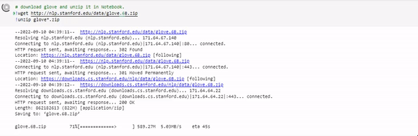

from tensorflow.keras.preprocessing.text import Tokenizer
from tensorflow.keras.preprocessing.sequence import pad_sequences
import numpy as np
  
x = {'the', 'match', 'score', 'prime',
     'player', 'manager', 'league'}
  
# create the dictionary.
tokenizer = Tokenizer()
tokenizer.fit_on_texts(x)
#define a utility function for embedding using glove
def embedding_for_vocab(file_path, word_index,
                        embedding_dimension):
    vocabulary_size = len(word_index) + 1
      
    # Adding again 1 because of reserved 0 index
    VocabEmbeddingMatrix = np.zeros((vocabulary_size,
                                       embedding_dimension))
  
    with open(file_path, encoding="utf8") as f:
        for line in f:
            word, *vector = line.split()
            if word in word_index:
                idx = word_index[word]
                VocabEmbeddingMatrix[idx] = np.array(
                    vector, dtype=np.float32)[:embedding_dimension]
  
    return VocabEmbeddingMatrix
  
  
# matrix for vocab: word_index
embedding_dimension = 50
VocabEmbeddingMatrix = embedding_for_vocab(
    'glove.6B.50d.txt', tokenizer.word_index,
  embedding_dimension)
  
print("Dense vector for first entry is => ",
      VocabEmbeddingMatrix[1])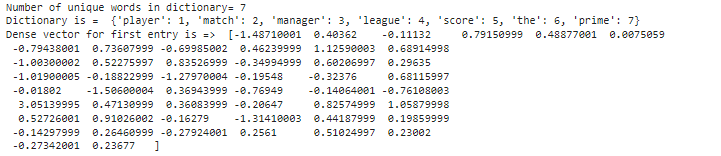

Google’s Word2vec

Google's Word2Vec contains models such as DBPedia vectors (wiki2vec) and Google News.

#download the model
!wget http://vectors.nlpl.eu/repository/20/51.zip
#unzip
!unzip 51.zip
#gzip the model for loading
!gzip model.bin

In this example, we use the model to obtain words with high cosine similarity with a list of words.

import gensim
from gensim.models import word2vec
from gensim.models import KeyedVectors
from sklearn.metrics.pairwise import cosine_similarity
EMBEDDING_FILE = 'model.bin.gz'
word_vectors = KeyedVectors.load_word2vec_format(EMBEDDING_FILE, binary=True)
#get most similar words in the word vector
result = word_vectors.most_similar(positive=['player', 'league'], negative=['man'])
most_similar_key, similarity = result[0]  # look at the first match
print(f"{most_similar_key}: {similarity:.4f}")

Fasttext

Install Fasttext glonnlp and mxnet.

pip install fasttext
pip install mxnet
pip install gluonnlp

You can access Fasttext pre-trained models using gluonnlp. Below is an implementation of the fastText embeddings trained on the wiki.simple dataset.

def tokenizer(source_str, token_delim=' ', seq_delim='\n'):
    import re
    '''Utility function for tokenizing'''
    tokens = filter(None, re.split(token_delim + '|' + seq_delim, source_str))
    return tokens
sentence = "The player scored twice during the match "
counter = nlp.data.count_tokens(tokenizer(sentence))
#create vocabulary
vocab = nlp.Vocab(counter)
#attach embedding
vocab.set_embedding(fasttext_model)
#check the embedding vector

vocab.embedding['player'][:5]

Hugging Face

Our TensorBoard guide demonstrated how to use Hugging Face for NLP tasks. You can use HuggingFace for problems related to:

• Question answering
• Summarization
• Translation
• Text generation

For instance, we might be interested in determining the named entities in a given text. To do so, we will use the BERT model with Huggin Face.

Install transformers:

pip install transformers sentencepiece

from transformers import AutoTokenizer, AutoModelForTokenClassification
from transformers import pipeline

tokenizer = AutoTokenizer.from_pretrained("dslim/bert-base-NER")
model = AutoModelForTokenClassification.from_pretrained("dslim/bert-base-NER")

nlp = pipeline("ner", model=model, tokenizer=tokenizer)
sentence = "The player scored twice during the match in Moscow and helped Brendan Rodgers manager win the league"
ner_results = nlp(sentence)
print(ner_results)

Transfer learning with PyTorch

PyTorch offers a range of deep learning functionalities, including pre-trained models. You can access a pre-trained model in PyTorch, as shown below.

import torchvision
model_conv = torchvision.models.resnet18(pretrained=True)

Check out additional implementations of transfer learning using PyTorch in the official documentation.

Transfer Learning for Computer Vision Tutorial — PyTorch Tutorials 1.12.1+cu102 documentation

How can you use pre-trained models?

Pre-trained neural networks can be used for prediction, feature extraction, and fine-tuning.

Let's explore these functions further.

Prediction

You can obtain a pre-trained model and use it for predictions without modification. The example below demonstrates the use of VGG16 for predicting the category of a rabbit.

from keras.preprocessing.image import load_img
# load an image from path
path = 'satyabratasm-u_kMWN-BWyU-unsplash.jpg'
img = load_img(path, target_size=(224, 224))
from keras.preprocessing.image import img_to_array
# convert the  pixels to a numpy array
img = img_to_array(img)

# reshape data for the pre-trained VGG model
img = img.reshape((1, img.shape[0], img.shape[1], img.shape[2]))

from keras.applications.vgg16 import preprocess_input
# transform the img for the pre-trained VGG model
img = preprocess_input(img)
# predict the probability for the output classes used in ImageNet
yhat = model.predict(img)
from keras.applications.vgg16 import decode_predictions
# convert the probabilities to discrete class labels
label = decode_predictions(yhat, top = 5)
# Get the most likely output with the highest probability
label = label[0][0]
# Show the predicted class
print('%s (%.2f%%)' % (label[1], label[2]*100))

Feature extraction

Consider the case of a VGG16 model with 16 layers and a VGG19 model with 19 layers. The figure below illustrates the architecture of a VGG16 model where the input layer accepts an image of dimensions (224 x 224 x 3) with an output of sigmoid prediction on the 1000 classes of ImageNet.

From the VGG16 model below, the input layer to the last max pooling layer (defined by 7 x 7 x 512) is considered the feature extraction part of the neural network. The remainder of the model is known as the classification function of the model.

Here's an implementation of the feature extraction process using a pre-trained VGG16 model.

import tensorflow as tf
from keras.applications.vgg16 import VGG16, preprocess_input
import numpy as np
#pre-trained model
model = VGG16(weights='imagenet', include_top=False)
#image for feature extraction
image_path = 'satyabratasm-u_kMWN-BWyU-unsplash.jpg'
image = tf.keras.utils.load_img(image_path, target_size=(224, 224))
from keras.preprocessing.image import img_to_array
image_data = img_to_array(image)

image_data = np.expand_dims(image_data, axis=0)
image_data = preprocess_input(image_data)

extracted_features = model.predict(image_data)

print (extracted_features.shape)

The extracted features can be used in additional machine learning tasks like clustering similar images and principal component analysis (PCA).

Fine-tuning

Fine-tuning is a transfer learning technique where we modify a model's output so that it learns about the new problem and train only the output of the model depending on this problem.

The process involves unfreezing the base model you have acquired  (or part of it) and re-training the model on the new problem's data with a very low learning rate.

Fine-tuning is aimed at improving the performance of the model. Since there are more parameters in the base model, some of which are related to other tasks, the process allows you to create feature representations from the base model such that the features are more relevant to your specified task.

# begin by unfreezing all layers of the base model
model.trainable = True

#Apart from the 10 last layers, freeze all the other layers
for layer in model.layers[:-10]: 
    layer.trainable = False

# compile and retrain with a very low learning rate
# compile and start training after freezing the layers
learning_rate = 1e-4
low_learning_rate = learning_rate / 100
#recompile the model with the new learning rate
model.compile(loss = 'binary_crossentropy',
              optimizer = tf.keras.optimizers.RMSprop(learning_rate = low_learning_rate), 
              metrics = ['acc']
)

You can adapt weights from the pre-trained model as initial weights for the model. There are no standard hyper-parameters that work for all transfer learning problems.

The best choice here depends on the new task. You might need to experiment with different approaches before settling on your task's optimal weights and hyper-parameters.

Example of transfer learning for images with Keras

We now know that the process of utilizing pre-trained models for similar tasks follows five general steps:

1. Obtain weights from a previously trained model.
2. Freeze the layers in the base model to retain the information learned during the original training of the base model.
3. Include additional trainable layers specific to the task on top of the frozen layers.
4. Train the new model on your dataset.
5. Fine-tune the base model using a low learning rate for potential improvement of the model's performance (optional).

Let's implement transfer learning using image and text data to practice what we have learned.

Transfer learning with image data

The theory behind transfer learning with images follows the argument that if a model is trained on a large and general enough dataset, the model can act as a generic model for other similar sub-tasks.

This approach is popular in computer vision and image detection. As we demonstrate in this section, it helps achieve relatively good results while reducing the time taken to train the model compared to training the model from scratch.

We will be working with the cat-dog dataset.  

Getting the dataset

The data can be obtained from TensorFlow datasets or downloaded from the dataset's repository. We will demonstrate both approaches.

#if the link below is broken, go to https://www.microsoft.com/en-us/download/confirmation.aspx?id=54765
#to obtain a new download link
!wget --no-check-certificate \
    "https://download.microsoft.com/download/3/E/1/3E1C3F21-ECDB-4869-8368-6DEBA77B919F/kagglecatsanddogs_5340.zip"
#remove previous files
!rm -rf PetImages
#unzip the dataset
!unzip -qq kagglecatsanddogs_5340.zip

Loading the dataset from a directory

Load the images using image_dataset_from_directory from TensorFlow.

from tensorflow.keras.preprocessing import image_dataset_from_directory
dir = "PetImages/"
data = image_dataset_from_directory(dir,
                                             shuffle=True,
                                             batch_size=32,
                                             image_size=(150, 150))

Alternatively, using TensorFlow datasets.

import tensorflow_datasets as tfds

#tfds.disable_progress_bar()

train_data, validation_data, test_data = tfds.load(
    "cats_vs_dogs",
    # Reserve 20% for validation and 10% for test
    split=["train[:40%]", "train[40%:50%]", "train[50%:60%]"],
    as_supervised=True,  # Include labels
)

print("There are %d training samples" % tf.data.experimental.cardinality(train_data))
print(
    "There are %d validation samples" % tf.data.experimental.cardinality(validation_data)
)
print("There are %d test samples" % tf.data.experimental.cardinality(test_data))

Plot samples images using Matplotlib.

plt.figure(figsize=(10, 10))
for i, (img, label) in enumerate(train_data.take(4)):
    ax = plt.subplot(2, 2, i + 1)
    plt.imshow(img)
    plt.title(int(label))
    plt.axis("off")
plt.suptitle("Sample images (Cat :0, Dog:1)")
plt.show()

Data pre-processing

Data pre-processing is an essential step in any machine learning pipeline. We have a small dataset. Therefore, it is advisable to initiate sample diversity by applying random but realistic transformations to the training data. Some of the transformations for image data include:

1. Random horizontal flipping or small random rotations
2. Gray-scaling
3. Shifts
4. Flips
5. Brightness
6. Zoom

These transformations are implemented through augmentation. Data augmentation helps to expose the model to different aspects of the training data, which helps to prevent overfitting. Keras provides various augmentation layers.

from tensorflow import keras
from tensorflow.keras import layers

data_augmentation = keras.Sequential(
    [layers.RandomFlip("horizontal"), #flips images 
     layers.RandomRotation(0.1),#randomly rotates images
     layers.RandomZoom(.5, .2), #randomly zooms images 
     layers.RandomFlip(
    mode="horizontal_and_vertical", seed=None #randomly flips images
)
]
)

The augmentation will be done during training. Below is a sample transformation on an image.

import numpy as np

for images, labels in train_data.take(1):
    plt.figure(figsize=(10, 10))
    first_image = images[7]
    for i in range(9):
        ax = plt.subplot(3, 3, i + 1)
        augmented_image = data_augmentation(
            tf.expand_dims(first_image, 0), training=True
        )
        plt.imshow(augmented_image[0].numpy().astype("int32"))
        plt.axis("off")
plt.suptitle("Sample preprocessed image")
plt.show();

Create a base model from the pre-trained Inception model

Obtain the Inception pre-trained model. We will use the InceptionV3 version of the Inception model. We initialize the model with saved weights and exclude the top layer (include_top=False) since it contains output information from the complete ImageNet dataset relevant to this task. The input shape is 150,150,3 because that is the size required by the Inception model.

base_model = keras.applications.InceptionV3(
    weights="imagenet",  # Load weights pre-trained on ImageNet.
    input_shape=(150, 150, 3),
    include_top=False,  #Exclude ImageNet classifier at the top
)

Remember, we want to use the saved knowledge in the base model. Therefore, we will freeze all layers, so they are not updated when compiling the model. Otherwise, we'd be training the model from scratch.

# Freeze the base_model
base_model.trainable = False

Create the final dense layer

We excluded the top layer when acquiring the InceptionV3 model. We will instead include a new final dense layer for the model.

Start by applying the augmentation strategies to the input images.  

#standardize the input
inputs = keras.Input(shape=(150, 150, 3))
x = data_augmentation(inputs)  # Apply random data augmentation

Pre-trained Inception weights expect the input to be scaled from (0, 255) (-1., +1.). For this, we will use the Rescaling layer.

#rescale
scale_layer = keras.layers.Rescaling(scale=1 / 127.5, offset=-1)
x = scale_layer(x)

Finally, we get to define the model:

1. Define the base model to run in inference mode to prevent updating the batch normalization layers (training=False).
2. Generate features from the base model using GlobalAveragePooling2D.
3. Apply dropout regularization.
4. Add a final dense layer.

x = base_model(x, training=False)
x = keras.layers.GlobalAveragePooling2D()(x)
x = keras.layers.Dropout(0.2)(x)  # Regularize with dropout
outputs = keras.layers.Dense(1)(x)
model = keras.Model(inputs, outputs)

model.summary()

The new dense layer has 1,281 parameters which we will be training in the next step.

The model is defined using the Keras Functional API.

Train the model

Time to train the model using the pre-processed data. As expected, the base model allows us to obtain relatively high accuracy.

First, compile the model to include the additional layer and train it over a few epochs. Define:

• An EarlyStopping callback to stop training if there is no improvement after three epochs.  
• A TensorBoard callback to track the model's performance.

from tensorflow.keras.callbacks import EarlyStopping, TensorBoard
!rm -rf image_logs
%load_ext tensorboard
log_folder = 'image_logs'
callbacks = [
            EarlyStopping(patience = 3),
            TensorBoard(log_dir=log_folder)
            ]

#compile the model to 
model.compile(optimizer='adam',
              loss=tf.keras.losses.BinaryCrossentropy(from_logits=True),
              metrics=keras.metrics.BinaryAccuracy())
hist = model.fit(train_data,
                 epochs=5, 
                 validation_data = validation_data, callbacks = callbacks)

The model attains an impressive 95.96% classification accuracy on the test data with a loss of approximately 0.1127.

#evaluate performance on test data
loss, accuracy = model.evaluate(test_data)
print("Fine-tuned model accuracy:", round(accuracy, 4)*100)
print("Fine-tuned model loss:", round(loss, 4))

%reload_ext tensorboard
%tensorboard --logdir {'image_logs/'}

Fine-tuning the model

Fine-tuning is an optional step aiming to improve the model's performance. However, fine-tuning has to be done with care because it is easy to overfit. Overfitting is prevented by setting a low learning rate.

First, unfreeze the layers you would like to re-train. In this case, unfreeze the last five layers.

#unfreeze the base model
base_model.trainable = False
#Apart from the 5 last layers, freeze all the other layers
for layer in model.layers[:-5]: 
    layer.trainable = True #unfreeze layers
model.summary()

Now we have more trainable parameters. The next step is to compile the model to update the parameters.

learning_rate = 1e-5
model.compile(
    optimizer=keras.optimizers.Adam(learning_rate),  # Low learning rate
    loss=keras.losses.BinaryCrossentropy(from_logits=True),
    metrics=[keras.metrics.BinaryAccuracy()],
)

Next, train the model on a few epochs and a low learning rate.

!rm -rf fine_tune_logs
%load_ext tensorboard
log_folder = 'fine_tune_logs'
callbacks = [
            EarlyStopping(patience = 5),
            TensorBoard(log_dir=log_folder)
            ]
epochs = 5
hist1 = model.fit(train_data,
          epochs=epochs,
          validation_data=validation_data,callbacks=callbacks)

To prevent overfitting, monitor the training loss using a callback such that the training stops when there is no improvement to the model performance after three epochs.

The model's performance improved slightly, with an accuracy of approximately 96% and a loss of 0.1049 on the test data.

#evaluate performance on test data
loss, accuracy = model.evaluate(test_data)
print("Fine-tuned model accuracy:", round(accuracy, 4)*100)
print("Fine-tuned model loss:", round(loss, 4))

%reload_ext tensorboard
%tensorboard --logdir {'fine_tune_logs/'}

Example of transfer learning with natural language processing

There are various types of transfer learning in natural language processing (NLP), including inductive and transductive learning.

In this section, we will see transfer learning in action for NLP.

Pretrained word embeddings

Pre-trained embeddings are embeddings learned from one problem and are subsequently used to solve a different but similar task. A word embedding is a learned representation of textual data in a vector space.

In word embeddings, words with the same meaning have similar representations. Therefore, you can use word embeddings from a different task on a new but similar task.

Training word embeddings on large datasets can take a lot of time besides consuming a lot of resources. Hence the need for using pre-trained word embeddings.

Some of the popular pre-trained word embeddings include:

1. Google’s Word2vec
2. Stanford’s GloVe

In this guide, we will demonstrate the application of Stanford’s GloVe in NLP problems and, more specifically, detecting sentiments.

Loading the dataset

First, let us acquire the sentiment dataset:

!wget !wget https://archive.ics.uci.edu/ml/machine-learning-databases/00462/drugsCom_raw.zip
!unzip drugsCom_raw.zip

Next, import the packages used in this task.

import pandas as pd
import tensorflow as tf
from tensorflow.keras.preprocessing.text import Tokenizer
from tensorflow.keras.preprocessing.sequence import pad_sequences
from tensorflow.keras.layers import Embedding, LSTM, Dense, Bidirectional, Dropout, SpatialDropout1D, GlobalAveragePooling1D
from tensorflow.keras.models import Sequential
import numpy as np
from sklearn.model_selection import train_test_split
import re
from tensorflow.keras.utils import to_categorical

Load the obtained data using Pandas and select the relevant variables for the task, i.e., review and sentiment category.

#read the data
df = pd.read_csv('drugsComTrain_raw.tsv', sep='\t')
#create sentiment column
df['category'] = [1 if int(x)>5 else 0 for x in df['rating']]
#get relevant variables
df = df[['review', 'category']].copy()
df.head()

The objective is to use learned embeddings to predict the category of the sentiments (ratings) of the reviews by various drug users. We will split the data and use 70% for training and the rest for model evaluation and testing.

First, let us pre-process the data.

Data pre-processing

Data pre-processing facilitates extracting the most relevant features from textual data, a process essential in all machine learning workflow regardless of the data type.

Vectorizing the words

The next step is to map the text data to a corresponding vector of real numbers. The resulting units are called token indices. These are numerical representations of the text data, i.e., reviews in this task.

Create a vectorization layer containing the vectors and the resulting vocabulary that will be used to generate a word index for the embedding matrix.

A quick examination of the data reveals that the sentences have varying lengths. This will be handled by padding the sentences to the same length max_length during vectorization.

df['words in sentence'] = [len(item.split()) for item in df.review]
df.head()

Create a vectorization layer that generates integer representations of the reviews.

import tensorflow as tf
max_features = 10000  # Maximum vocabulary size.
max_len = 100 # Sequence length to pad the outputs to.
vectorize_layer = tf.keras.layers.TextVectorization(standardize='lower_and_strip_punctuation',max_tokens=max_features,output_mode='int',output_sequence_length=max_len)
vectorize_layer.adapt(list((df['review'].values)),batch_size=None)

Below is a sample integer representation of the first sentence in the train data

X_train[0]

Apply the vectorization layer to train and test sets

#split the data into train and test sets
from sklearn.model_selection import train_test_split
X_t = list((df['review'].values))
X_train, X_test , y_train, y_test = train_test_split(X_t, y , test_size = 0.30)
#apply cetorization layer to train and test
X_train =  vectorize_layer(X_train)
X_test =  vectorize_layer(X_test)

Using GloVe Embeddings

GloVe embeddings are generally used in NLP tasks. These embeddings can be obtained as shown below.

#download glove embeddings
# download glove
!wget http://nlp.stanford.edu/data/glove.6B.zip
# unzip it in Notebook
!unzip glove*.zip

Unzip the embeddings into your workspace.

# unzip it in Notebook
!unzip glove*.zip

Create your embedding index using the collected word embeddings.

#load your embeddings
embeddings_index = {}
emb = open('glove.6B.100d.txt')
for sentence in emb:
    values = sentence.split()
    word = values[0]
    coefs = np.asarray(values[1:], dtype='float32')
    embeddings_index[word] = coefs
emb.close()

print('There are %s word vectors.' % len(embeddings_index))

Create the embedding layer

First, create a custom word_index from the vectorizer's vocabulary.

#get vocabulary
voc = vectorize_layer.get_vocabulary()
#create a word index
word_index = dict(zip(voc, range(len(voc))))

Using the resulting dictionary, create an embedding matrix for all the words in the training set using the embedding_index.

num_tokens = len(voc) + 2
embedding_dim = 100
hits = 0
misses = 0

# Prepare embedding matrix
embedding_matrix = np.zeros((num_tokens, embedding_dim))
for word, i in word_index.items():
    embedding_vector = embeddings_index.get(word)
    if embedding_vector is not None:
        # Words not found in embedding index will be all-zeros.
        embedding_matrix[i] = embedding_vector
        hits += 1
    else:
        misses += 1

Now you can define an embedding layer using the pre-trained embeddings by applying the following settings:

• input_dim : Size of the vocabulary.
• embeddings_initializer : The embedding matrix that you defined.
• output_dim : Length of the vector for each word.
• trainable : Set to false to avoid losing the information in the pre-trained embedding.

from tensorflow.keras.layers import Embedding
from tensorflow import keras

embedding_layer = Embedding(
    input_dim = num_tokens,
    output_dim = embedding_dim,
    embeddings_initializer=keras.initializers.Constant(embedding_matrix),
    trainable=False,
)

Create the model

You can define your model using the resulting embedding layer. We use the Bidirectional LSTMs to pass information backward and forward.

Next, create the model.

# define model
from tensorflow.keras.layers import Flatten
model = Sequential()
vocab_size = 10002
#use the embedding_matrix
e = Embedding(vocab_size, 100, weights=[embedding_matrix], input_length=100, trainable=False)
model.add(e)
model.add(Bidirectional(LSTM(10, return_sequences=True, dropout=0.1, recurrent_dropout=0.1)))
model.add(Flatten())
model.add(Dense(2, activation='sigmoid'))
# compile the model
model.compile(optimizer='adam', loss='binary_crossentropy', metrics=['accuracy'])
# summarize the model
print(model.summary())

Training the model

Time to compile and train the model. You can use your preferred metric to evaluate the performance of the model. In this implementation, we are using the accuracy metric.

After compiling, we use callbacks to monitor the model's performance and stop the training process if it fails to improve after three epochs.

%load_ext tensorboard
!rm -rf embed_logs
log_folder = 'embed_logs'
from tensorflow.keras.callbacks import EarlyStopping, TensorBoard
#apply callbacks
callbacks = [
            EarlyStopping(patience = 3),
            TensorBoard(log_dir=log_folder)
            ]
#compile
model.compile(loss='binary_crossentropy',optimizer='adam',metrics=['accuracy'])
num_epochs = 10
history = model.fit(X_train, y_train, epochs=num_epochs, validation_data=(X_test, y_test),callbacks=callbacks, batch_size = 2560)

The model begins with an accuracy of 70.63% on the validation and attains an accuracy of approximately 79.21% on the test set, respectively, which is arguably a decent performance since we did not have to train the embeddings from scratch.

You can visualize your events using TensorBoard, as shown below.

%reload_ext tensorboard
%tensorboard --logdir {'embed_logs/'}

Final thoughts

With the advent of technologies like big data and deep learning, there is a pressing need to adopt new methodologies that facilitate the fast development of optimally performing models. Transfer learning, as demonstrated in this guide, provides the right resources to implement better models in image classification and natural language processing tasks with relative ease compared to training the models from scratch. In particular, you have learned:

• What is transfer learning?
• Types of transfer learning.
• Steps of implementing transfer learning.
• Where to find transfer learning models.
• How to use pre-trained models for transfer learning.
• How to implement transfer learning in an image classification task.
• Using transfer learning to solve a natural language processing task.    

Want to explore TensorFlow further? Check these articles on our blog:

• TensorBoard tutorial (Deep dive with examples and notebook)
• Object detection with TensorFlow 2 Object detection API
• How to train deep learning models on Apple Silicon GPU
• How to build CNN in TensorFlow(examples, code, and notebooks)
• How to build artificial neural networks with Keras and TensorFlow
• Custom training loops in Keras and TensorFlow
• Flax vs. TensorFlow
• How to build TensorFlow models with the Keras Functional API
• TensorFlow Recurrent Neural Networks (Complete guide with examples and code)

Other resources

• gensim
• Download pre-trained word vectors

Follow us on LinkedIn, Twitter, GitHub, and subscribe to our blog, so you don't miss a new issue.